The theory of dispersion of light waves is well known and can be found in many textbooks, as for example [1–3], but the way it is usually presented deserves some comments. For example, causality can be seen as not being fully respected in the basic equations, within the meaning of causal link between their parameters.

This paper also emphasizes that the indexes are very convenient to understand more easily the equations describing dispersion. They should be viewed as inverses of velocity, normalized to 1/c, the inverse of light velocity c in a vacuum, knowing that there is no short word for these inverses that are involved in these equations. Furthermore, indexes are dimensionless values, which avoids dealing with units that are not always easily understandable, as we shall see.

In addition, two simple and amusing geometrical constructions are presented to derive group index n_g from refractive index n with a tangent. To my knowledge, they are original. They apply to material dispersion, but also to guidance dispersion in a fiber or a waveguide, as well as to birefringence and intrinsic polarization mode dispersion (I-PMD) in polarization-maintaining (PM) fibers or birefringent waveguides.

Obviously, this does not prevent the use of Sellmeier’s equation [4] and derivatives with a computer, to calculate precisely these indexes, but this brings a complementary view to visualize simply the question of dispersion, and the relationship between refractive index n and group index n_g.

The first analysis of dispersion was done by Newton, in the mid-17th century, with a prism that can separate the various colors of white light, because the refractive index n (or index of refraction) of a glass is not constant; it is called chromatic dispersion (chroma is color, in ancient Greek). At the beginning of the 19th century, with the work of Fresnel on the mathematical theory of diffraction, it was finally accepted by the scientific community that light is a wave, as proposed by Huygens at the end of the 17th century, and that the index n is the ratio between light velocity c in a vacuum and its lower velocity in a medium. Remember that Newtonian corpuscular theory stated the opposite, with light going faster in a medium than in a vacuum, and that it required more than a century to get Huygens’ wave model accepted, because of the tremendous prestige of Newton, as discussed by Aspect in a recent historical review paper [5].

In acoustics, it was proposed by Hamilton in the first half of the 19th century that a modulated wave has in fact two velocities: the sinusoidal carrier does propagate at the velocity of a continuous wave, called the phase velocity v_φ, but the modulation term propagates at the so-called group velocity v_g. This concept of group velocity was later developed in full mathematical details by Rayleigh in his iconic book, The Theory of Sound [6], and group velocity was seen as the velocity of signal energy.

At the beginning of the 20th century, the application of this concept to optical waves raised many questions, because it could lead to a group velocity higher than c, in the case of high Anomalous dispersion, i.e., when (dn/dλ) ≫ 0, which was contradictory with the Theory of Relativity. This question was brilliantly solved by Sommerfeld and Brillouin in twin papers of 1914 [7, 8]. An English version of these papers can be found in the very interesting Brillouin’s book of 1960, Wave Propagation and Group Velocity [9]. The important result is that anomalous dispersion happens when there is absorption, as in the far ultra-violet for example, but with absorption, group velocity is not the velocity of signal energy anymore; then, it is not contradictory with Relativity.

Going back to the usual case of normal optical dispersion in transparent dielectric media, i.e., when (dn/dλ) < 0, phase velocity v_φ = c/n and group velocity v_g are classically given by [1–3]:(1)vφ = ω/km and vg = dω/dkm,where ω is the angular (temporal) frequency, and k_m is the angular spatial frequency in the medium. For k_m = 2π/λ_m = 2π · n/λ, with λ_m = λ/n being the wavelength in the medium and λ being the wavelength in a vacuum, the terms angular wave number, or wave number alone, are also used, but I prefer angular spatial frequency to outline the duality between the temporal domain and the spatial domain.

I do not like much the use of the derivative dω/dk_m for the definition of v_g, since it does not respect the causal link between k_m and ω, that I call, in short, causality in this paper: it is k_m that depends on ω, and not ω that depends on k_m. You may say that dω/dk_m and (dk_m/dω)⁻¹ are alike for Leibniz’s notation of derivatives, beauty of math, but with Lagrange’s notation, that I prefer here, it is less clear: ω′(k_m) suggests a causality that would not be fully respected, whereas [k′_m(ω)]⁻¹ does respect causality.

To be more specific, you must agree that it is the index n (involved in k_m = 2π · n/λ), that depends on the wavelength λ in a vacuum (involved in ω, with ω = 2π · c/λ), and not the opposite; it is n(λ) and not λ(n), even if λ, as a function of n, remains mathematically possible. Math does not care about causality and can inverse a function, but causality is fundamental in physics! Equation (1) should be:(2)1/vφ = km/ω and 1/vg=dkm/dω = k'm(ω).

You may think that it is nit-picking but, to me, it is important, and I wanted to share this view. I am not the only one to think that, and equation (2) is found in several textbooks [10–12], even if they do not outline the difference between (1) and (2). It must be obvious for the authors of these references, but I am not sure that it is obvious for every reader of this article.

Now, if a frequency is the inverse of a period, as we have all learned with music, there is no short word for the inverse of a velocity, that is involved in (2). The habit is to use temporal delay over a unit distance [3] or group delay per unit length [10], with t_g = 1/v_g, but it is not very concise. Slowness could have been possible, but it is not very positive wording. This can be overcome with the use of refractive index n, also called phase index since n = c/v_φ, and of group index n_g = c/v_g. They should be viewed as the inverse of a velocity, normalized to 1/c. Relativity physicists do normalize the time dependence c · t of their equations with c = 1, to get the same temporal dimension as that of the spatial coordinates; we can do the inverse! So, there are:(3)n = (1/vφ)/(1/c) and ng = (1/vg)/(1/c).

You may think that it is nit-picking again, or obvious math, but I prefer to consider that it is useful to understand dispersion better. Using group index n_g, as defined in (3), it is simple to derive its relationship with phase index n. Since k_m = n(ω)·ω/c, there is:(4)ng(ω) = (1/vg)/(1/c) = c· dkm/dω = d[nω·ω]/dω.

It is important to notice in (4) the derivative of the product [n(ω) · ω]. It explains the difference between dispersion seen as a function of wavelength λ, and seen as a function of angular frequency ω, as we shall see later. Now from (4):(5)ng(ω) = d[nω·ω]/dω=n(ω) + [ω·dn/dω].

With Lagrange’s notation of derivative, instead of Leibniz’s notation, this yields:(6)ngω= nω+ ω·n'ω.

This well-known equation is often written as a function of the wavelength λ in a vacuum. Since ω = 2π · c/λ, there is, by logarithmic differentiation, dω/ω = −dλ/λ, and then:(7)ng(λ) = n(λ) - [λ ·dn/dλ]or, with Lagrange’s notation:(8)ngλ= nλ- λ·n′λ.

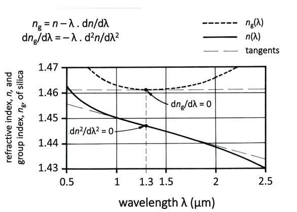
It is often taught that there is no group velocity dispersion, when the second derivative n″(λ), or d²n/dλ², is equal to 0; for silica fibers, it is for λ = 1.3 μm. Geometrically, this corresponds to an inflexion point of the refractive index curve n, as a function of wavelength λ (Fig. 1). It is mathematically true but, again, it does not fully respect causality. The cause is that there is no group dispersion when group velocity v_g, as well as group index n_g, are constant, i.e., when its first derivative dn_g/dλ, or n′_g(λ), is equal to zero. It happens to be the case when the second derivative of the refractive (or phase) index, d²n/dλ², or n″(λ), equates zero, but it is only a consequence of the fact that dn_g/dλ = −λ · d²n/dλ²; it is not the original cause which is dn_g/dλ equates zero.

This result influenced a vocabulary that must be handled with care. Chromatic dispersion, also known as phase velocity dispersion, i.e., first derivative of phase index dn/dλ ≠ 0, is often called first-order dispersion, and group velocity dispersion, i.e., first derivative of group index dn_g/dλ ≠ 0, but also second derivative of phase index d²n/dλ² ≠ 0, is often called second-order dispersion.

So, I have another comment: if one considers frequencies (angular, ω, or regular temporal, f = ω/2π, or spatial, σ = 1/λ), this does not work anymore; this works only with period, i.e., wavelength λ or temporal period T = 1/f. No group velocity dispersion means that dn_g/dω (or dn_g/df, or dn_g/dσ) is equal to zero, since it is the basic cause, but from (5):(9)dng/dω = d[n(ω) + (ω· dn/dω)] = (2·dn/dω) + (ω· d2n/dω2)

Therefore, when dn_g/dω = 0, the second derivative d²n/dω² of the phase index equates −(2·dn/dω)/ω, and it is not null. There are similar equations with f and σ, since df/f = dσ/σ = dω/ω, by logarithmic differentiation.

Nevertheless, it is possible to view second-order dispersion with frequency. It is not as visual as for wavelength, with the inflexion point of the refractive index dependence, but it remains simple mathematically. We saw in (2) that t_g = 1/v_g = dk_m/dω, and group dispersion is the first derivative of this group delay t_gover a unit distance, i.e., 1/v_g. With frequency, it is called group velocity dispersion (GVD), and:(10)GVD = dtg/dω = d(1/vg)/dω = d2km/dω2.

Since k_m = 2π · n/λ = [(n(ω)·ω]/c, there is no second order dispersion when the second derivative of the product n(ω) · ω is null, i.e., when d² k_m/dω² = (1/c)·d²[n(ω)·ω]/dω² = 0, whereas, with λ, it is when the second derivative of the refractive index n(λ) alone is null, i.e. d²n/dλ², as we already saw.

To promote, again, indexes as normalized inverse velocities, I have an additional comment with what is called group dispersion parameter, D, and what is called, we just saw, group velocity dispersion, GVD, as you find on refractiveindex.info web site, for example. D is classically expressed in ps/(nm km), and it is simply [3]:(11)D=dtg/dλ = d(1/vg)/dλ.

Using the first derivative of n_g(λ), this yields:(12)D = (1/c)· dng/dλ = (1/c)·n′g(λ).

GVD is similar, but it is using the derivative with respect to ω, instead of λ:(13)GVD = dtg/dω = d(1/vg)/dω.

Using the first derivative of n_g(ω), this yields:(14)GVD = (1/c) · dng/dω = (1/c) ·n′g(ω).

Its unit is square second per meter. This is concise but not easily understandable. It would be clearer to use s/[(rad/s) m], or s²/(rad m), a radian per second being the unit of ω, even if a radian is a dimensionless unit that can be omitted. This is a complicated question, by the way, to decide if a dimensionless unit can be omitted or not?

In silica, at 1550 nm, dn/dλ ≈ −0.012 μm⁻¹ and dn_g/dλ ≈ +0.007 μm⁻¹ (Fig. 2). I like these values that have a simple unit, and that you can check on index curves. Now, since 1/c is about one nanosecond per foot (a very useful value that I learned and still remember from my postdoc at Stanford University, in the early 1980s), group dispersion parameter D is about +23 ps/(nm km), and group velocity dispersion GVD is about −28 ps²/km (or fs²/mm).

To understand better ps²/km, the unit of GVD, and to compare it with ps/(nm km), the unit of D, one must see that in “ps²”, there are a first “ps” for the delay, as in ps/(nm km), and a second “ps” that is actually 1/(10⁺¹² rad/s), with the omission of dimensionless radian. At 1550 nm, where the temporal frequency f is 193.5 THz, the angular frequency, ω = 2π · f, is about 1.2 × 10⁺¹⁵ rad/s; then, a value of 10⁺¹² rad/s for the shift ∆ω, is around 0.1% of ω. The “nm” used in D for ∆λ is also a shift of about 0.1% of the wavelength, that is in the μm range, and then, the two numerical values, 23 and 28, are close. One femtosecond, for GVD, is about equivalent to one nanometer to the −1 power, for D.

In any case, ps²/km remains a strange unit to me. As a teaser, it would have been also possible to use a concise and strange unit for D: ps/mm², since 1 nm × 1 km = 1 mm × 1 mm, but with mm², it looks like an area!

Finally, remember that D and GVD have opposite signs, since ω = 2π · c/λ, and then, dω/dλ is negative, as well as dλ/dω. To talk about positive or negative group dispersion requires to specify if it is with respect to period, or to frequency. To avoid this problem, it is customary to use for group velocity dispersion the same vocabulary as the one used for phase velocity dispersion. As we saw, normal dispersion corresponds to a negative derivative of the index with respect to λ, and anomalous dispersion corresponds to a positive derivative. However, I am not very fond of this vocabulary for group dispersion, even if it is convenient. Anomalous has an understandable meaning with phase velocity dispersion, since it is when the medium is absorbing, and it is not the normal use in the transparency window. With group velocity dispersion, a positive group index derivative is not Anomalous, nor abnormal, strictly speaking. Taking the case of silica, it is simply above 1.3 μm, as seen in Figure 2!

Let us consider the theoretical case of a material without any group dispersion. As we saw, dn_g/dλ = 0 implies that d²n/dλ² = 0. The curve of the refractive (or phase) index n as a function of wavelength λ is a simple affine function, with a constant slope, equal to dn/dλ, since d²n/dλ² = 0:(15)n(λ) = n(0) + (λ· dn/dλ).

Because the group index n_g(λ) is equal to n(λ) – (λ · dn/dλ), as seen in (7), there is:(16)ngλ= n0+ λ·dn/dλ– λ ·dn/dλ= n0.

Group index n_g is constant and equal to the value n(0) of the phase index for a null wavelength (Fig. 3).

As it can be simply visualized with this Figure 3, normal dispersion, i.e., a negative slope dn/dλ, yields a group index n_g higher than the phase index n. Conversely, anomalous dispersion, i.e., a positive slope dn/dλ, yields a group index n_g lower than the phase index n, and one can easily understand that with a steep positive slope, group index can become lower than one, and even negative, which was obviously a problem with the theory of Relativity, but this was solved by Sommerfeld and Brillouin, as we already saw [7–9].

Now, with the practical case of a material with group dispersion, one must consider the tangent to the curve n(λ). Using Lagrange’s notation, which is clearer, here, than Leibniz’s notation, the equation T₀(λ) of this tangent, for a given wavelength λ₀, is:(17)T0λ = nλ0+ n′λ0· λ - λ0.

Then, it is simple to see with (7) again, that for a null wavelength:(18)T0(0) = n(λ0) - [n'λ0· λ0] = ng(λ0).

The tangent T₀(λ) to the curve n(λ), at λ₀, crosses the ordinate axis, i.e., when λ is zero, at the value n_g(λ₀) of the group index for λ₀ (Fig. 4). It is simple math, but it is amusing and, also, very useful to visualize simply the relationship between n and n_g.

Knowing this, Figure 1 can be revisited, even if silica is not transparent anymore below 0.15 μm (Fig. 5). Mathematically, it remains possible to continue the tangent toward zero. Math does not care about causality, as we already saw, nor does it care about transparency!

As we saw, a CW light wave propagates at a phase velocity v_φ = ω/k_m(ω), in a bulk medium. In an optical fiber, there are discrete modes that propagate at different phase velocities v_φi = ω/β_i(ω), where β_i(ω) is called the propagation constant of mode i [2, 3, 10]. These propagation constants depend on the angular temporal frequency ω, and they have an intermediate value between the angular spatial frequency k_m2 in the cladding of refractive index n₂, and k_m1, the one in the core of refractive index n₁. In the single-mode regime, the high-order modes are above cut-off, and the fundamental mode is the only one that can propagate. Its propagation constant β(ω) follows:(19)km2 = 2π·n2/λ < β(ω) < km1 = 2π·n1/λ.

It is very convenient to use the so-called effective index n_eff of the mode defined with:(20)β(ω) = 2π·neff(ω)/λ.

Following (19), n_eff has an intermediate value between n₂ and n₁, and like β it depends on frequency:(21)n2 < neffω< n1.

The angular (temporal) frequency ω is very useful to shorten mathematical equations, but everybody is more familiar with the wavelength λ in a vacuum. You know what is 1 μm, whereas 1 rad/s is not that obvious, besides the fact that it corresponds to 0.16 Hz. Therefore, the frequency dependence of n_eff is classically presented with respect to λ_c/λ, where λ_c is the cut-off wavelength of the second-order mode. This ratio does correspond to a frequency: it is the spatial frequency 1/λ normalized to 1/λ_c.

This effective index n_eff is a phase index, and all the mathematical equations of Section 2 can be used to find the effective group index n_g-eff. It is also possible to use the geometrical construction of Section 3, that relates a group index to its corresponding phase index.

The way to proceed is to invert the classical curve n_eff(λ_c/λ), and to get the inverted curve n_eff(λ/λ_c), that depends on λ, and not on 1/λ anymore (Fig. 6).

It is interesting to notice that this inverted curve is easier to understand, for the fundamental mode, than the classical one: as the wavelength increases, the mode widens [2], and it expands more in the cladding, which decreases the effective index n_eff. However, the classical representation remains better with several modes, since their effective index curves are spread about evenly in frequency, which would not be the case with the inverted representation.

Now, once you have this inverted representation in wavelength, you must just apply the geometrical construction of Figure 4, to find the value of the effective group index n_g-eff (Fig. 7).

Note, however, that it is possible to find also a geometrical construction with the frequency dependence. It is not as simple as with the period dependence, but it has some interest. The equation of the tangent T₀(ω) to the curve n(ω), for a given angular frequency ω_0, is:(22)T0ω = nω0+ ω - ω0· n′ω0,(23)T0(ω) = T0(0) + [(ω · n′(ω0)]with:(24)T00 = nω0- ω0 · n′ω0.The slope of this tangent is n′(ω₀).

Consider now the affine function DS₀(ω) starting from T₀(0), and having a double slope, i.e., a slope equal to twice that of the tangent T₀(ω):(25)DS0(ω) = T0(0) + 2 [ω·n′ω0.

Following (24), there is:(26)DS0ω0 = nω0+ ω0 · n′ω0.

As seen in (6), the group index follows n_g(ω) = n(ω) + [ω · n′(ω)], then:(27)DS0ω0 = ngω0.

With λ, we saw that the tangent to the curve n(λ), at λ₀, crosses the ordinate axis at n_g(λ₀). With ω, one draws a double-slope line DS₀(ω) (Fig. 8). In the case of the fundamental mode of a fiber, the double-slope construction can be used with the classical curve n_eff(λ_c/λ) seen in Figure 6a, as shown in Figure 9.

Obviously, this geometrical construction can also be used for high-order modes, as well as for integrated-optic waveguides.

The use of phase and group indexes as normalized inverses of velocity, as well as the geometrical constructions, that were presented, are also very useful for birefringence and intrinsic polarization mode dispersion (intrinsic PMD) [3] of high-birefringence polarization-maintaining (PM) fibers.

Phase birefringence B, or modal birefringence, or simply birefringence, is the difference between the phase effective index n_slow of the slow polarization mode, and n_fast, that of the fast mode. In addition, it is very convenient to use the concept of group birefringence B_g, instead of intrinsic PMD; this simplifies equations. B_g is the difference between the group indexes n_g-slow and n_g-fast:(28)B = nslow - nfast and Bg = ng-slow-ng-fast.

We saw in (7), that n_g(λ) = n(λ) – (λ · dn/dλ), then:(29)Bg(λ) = [nslow(λ) – (λ·dnslow/dλ)] - [nfast(λ) – (λ · dnfast/dλ)],(30)Bg(λ) = [nslow(λ) - nfast(λ)] – [λ·(dnslow/dλ - dnfast/dλ)],(31)Bg(λ) = B(λ) – [λ · dB/dλ].

This last equation (31) is similar to (7), replacing the indexes by the birefringences, therefore the geometrical construction, that we saw in Figure 4, can be used (Fig. 10).

The intrinsic PMD_i of high-birefringence PM fibers is the difference between the group delays per unit length of both modes [3]:(32)PMDi = tg-slow - tg-fast = (1/vg-slow) - (1/vg-fast) = (ng-slow/c) - (ng-fast/c),which yields a very simple equation:(33)PMDi = Bg · 1/c = [B – (λ·dB/dλ)] · 1/cknowing that 1/c is about one nanosecond per foot, as we already saw. Group birefringence is actually what is called intrinsic PMD, but normalized to 1/c. Typical group birefringence B_g of PM fibers is around 5 × 10⁻⁴, and again it is a dimensionless value, which yields an intrinsic PMD on the order of 1.5–2 ps/m.

Intrinsic PMD is related to phase birefringence dispersion: when dB/dλ ≠ 0, group birefringence B_g is different from phase birefringence B; it is a first-order dispersion. There is in addition group birefringence dispersion, when the first derivative dB_g/dλ ≠ 0. As with group index, it is also when the second derivative d²B/dλ² ≠ 0, since dB_g/dλ = −λ · d²B/dλ². It is a second-order dispersion that must be considered in certain cases as, for example, with optical coherence-domain polarimetry (OCDP) also called distributed polarization crosstalk analysis (DPXA) [13, 14].

This paper presents comments and geometrical constructions that should ease the understanding of dispersion, which is not always explained simply in textbooks. The points to remember are:

Group velocity is classically given with v_g = dω/dk_m, i.e., ω′(k_m), but this equation does not fully respect causality, within the meaning of causal link between its parameters.

I hope that this paper will be useful and help to clarify the subject. It is just based on what I had not fully understood about dispersion, over the forty-five years of my career, as you can check in [15, 16], where I classically used (1). I understand it better today, and I wanted to share it. And as you did notice, I do like the simple and amusing geometrical constructions with the tangent, which is the reason for this paper, even if I did not resist adding some comments that might look slightly provocative, but nevertheless important, I think.