
P. Bradford, N. C. Woolsey, G. G. Scott, G. Liao, H. Liu, Y. Zhang, B. Zhu, C. Armstrong, S. Astbury, C. Brenner, P. Brummitt, F. Consoli, I. East, R. Gray, D. Haddock, P. Huggard, P. J. R. Jones, E. Montgomery, I. Musgrave, P. Oliveira, D. R. Rusby, C. Spindloe, B. Summers, E. Zemaityte, Z. Zhang, Y. Li, P. McKenna, D. Neely, "EMP control and characterization on high-power laser systems," High Power Laser Sci. Eng. 6, 02000e21 (2018)
- High Power Laser Science and Engineering
- Vol. 6, Issue 2, 02000e21 (2018)
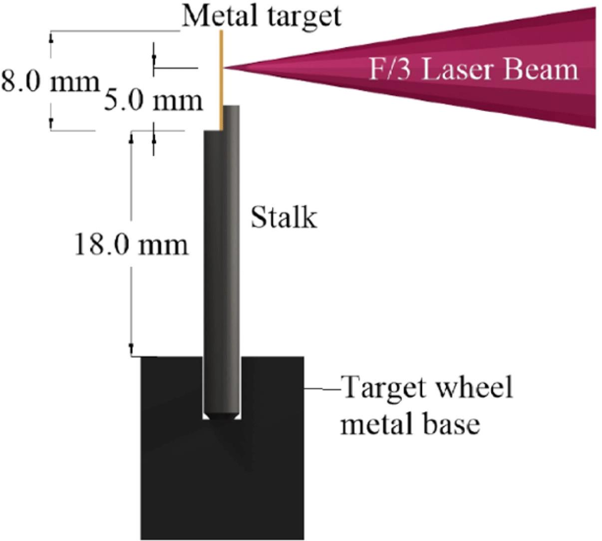
Fig. 1. Schematic of target design and experimental arrangement.
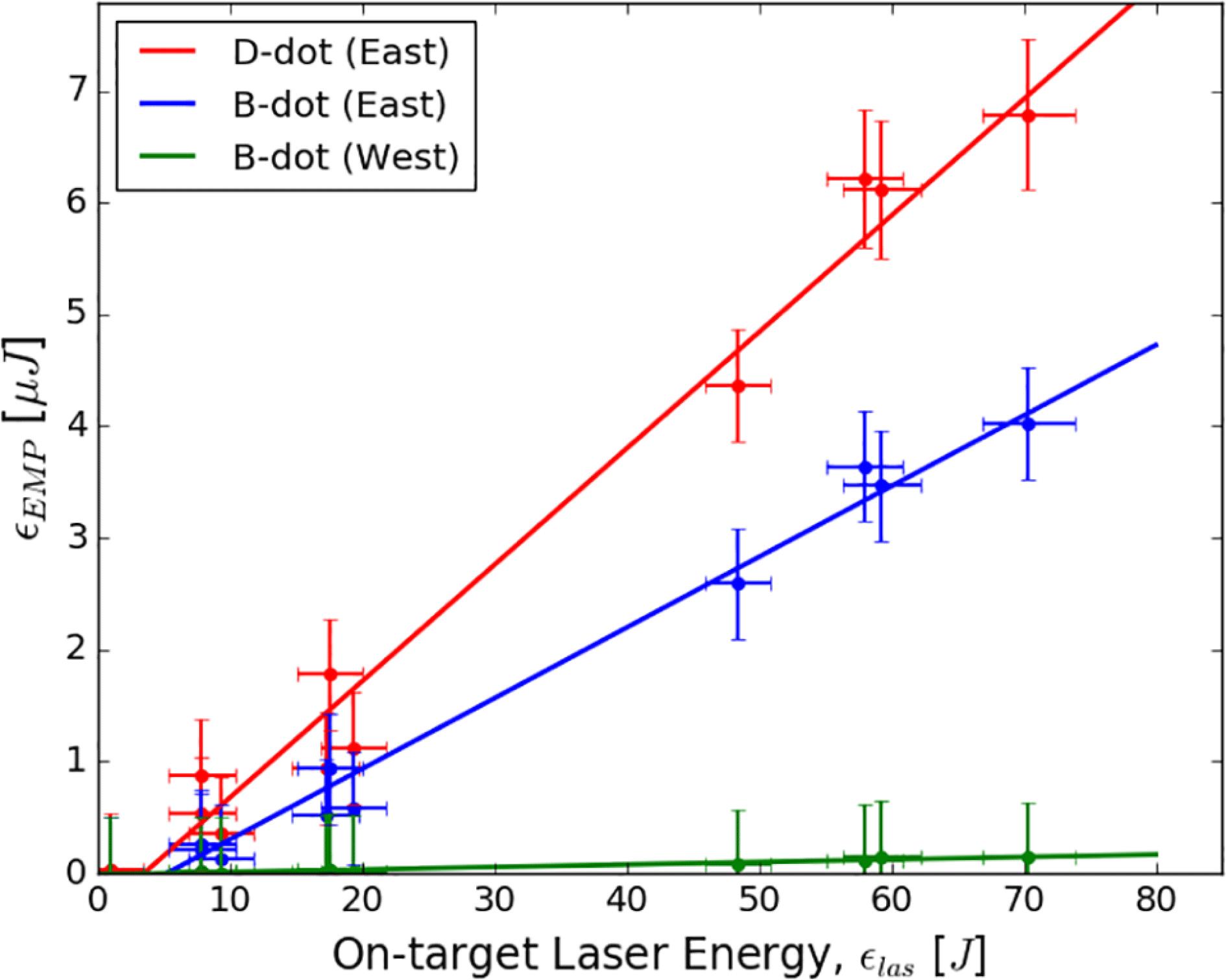
Fig. 2. EMP energy versus on-target laser energy for the D-dot and two B-dot probes. The coloured lines represent linear fits for all three probes.
Fig. 3. Plot of EMP energy and total number of escaping electrons versus laser pulse duration. The grey diamonds represent the ratio of EMP energy to on-target laser energy, while the orange diamonds represent the ratio of total electron number ( ) to on-target laser energy. EMP data was taken from the B-dot West probe.
) to on-target laser energy. EMP data was taken from the B-dot West probe. Fig. 4. EMP energy as a function of pre-pulse delay, measured by the D-dot probe.
Fig. 5. The ratio of EMP energy to laser energy plotted against defocus (as measured by the D-dot East probe). The Gaussian fit is meant as a visual aid, with a laser focal intensity of approximately  at the Gaussian peak.
at the Gaussian peak. Fig. 6. EMP energy as a function of on-target laser energy for wire, flag and standard foil designs (B-dot probe East). Laser focal intensity ranges from  to
to  on these shots and we have chosen a logarithmic
  -axis to emphasize the drop in EMP. Notice how changing the wire diameter has led to a deviation from the linear relationship between EMP and on-target laser energy.
to on these shots and we have chosen a logarithmic -axis to emphasize the drop in EMP. Notice how changing the wire diameter has led to a deviation from the linear relationship between EMP and on-target laser energy. Fig. 7. EMP energy versus on-target laser energy for a variety of different stalk designs (B-dot probe East). Laser focal intensity is between  and
and  for these shots. Also included is a linear fit to the standard CH cylindrical stalk data, as detailed in Figure
 2 .
and for these shots. Also included is a linear fit to the standard CH cylindrical stalk data, as detailed in Figure Fig. 8. The three different stalk designs: (a) standard cylindrical geometry with a geodesic path length of 20 mm; (b) a sinusoidally modulated stalk with the same maximum cross-section as the standard cylinder and a path length of 30 mm; (c) spiral stalk design with an identical diameter to (a), but a geodesic path length of 115 mm.
Fig. 9. Total number of electrons recorded by the electron spectrometer as a function of on-target laser energy. Uncertainties in on-target laser energy are  .
.
. Fig. 10. Number of electrons with energies above 5 MeV versus on-target laser energy. Uncertainties in on-target laser energy are  .
.
. Fig. 11. Side elevation of stalk designs used in 3D PIC simulations. Transparent grey sections represent a perfect electrical conductor (PEC), while the grey-green regions represent Teflon plastic. (a) Standard cylindrical stalk configuration: pure Teflon and PEC models were used. (b) Sinusoidally modulated Teflon stalk. (c) Teflon spiral stalk. (d) Half-length Teflon and PEC stalk.
Fig. 12. Two tables containing values of the magnetic component of the EMP energy ( ) at positions
  and
and  in the simulation box.
) at positions and in the simulation box. 

Set citation alerts for the article
Please enter your email address

© Copyright 2018-2021 | Chinese Laser Press. All Rights Reserved 沪ICP备15018463号-20