Computing plays an increasingly vital role in constructing intelligent, digital societies. The exponentially growing power consumption of digital computers brings some important challenges for large-scale computing. Optical computing can potentially provide advantages in terms of power efficiency, processing speed, and parallelism. Motivated by these, we have witnessed various research and development efforts on advancing optical computing over the last few decades.1^–32 Synergies between optics and machine learning have enabled the design of novel optical components using deep-learning-based optimization,33^–44 while also allowing the development of advanced optical/photonic information processing platforms for artificial intelligence.5^,20^–32^,45

Among different optical computing designs, diffractive optical neural networks represent a free-space-based framework that can be used to perform computation, statistical inference, and inverse design of optical elements.22 A diffractive neural network is composed of multiple transmissive and/or reflective diffractive layers (or surfaces), which leverage light–matter interactions to jointly perform modulation of the input light field to generate the desired output field. These passive diffractive layers, each containing thousands of spatially engineered diffractive features (termed as “diffractive neurons”), are designed (optimized) in a computer using deep-learning tools, e.g., stochastic gradient descent and error backpropagation. Once the training process converges, the resulting diffractive layers are fabricated to form a passive, free-space optical processing unit that does not consume any power except the illumination light. This framework is also scalable, since it can adapt to changes in the input field of view (FOV) or data dimensions by adjusting the size and/or the number of diffractive layers. Diffractive networks can directly access the 2D/3D input information of a scene or object and process the optical information encoded in the amplitude, phase, spectrum, and polarization of the input light, making them highly suitable as intelligent optical front ends for machine-vision systems.

Diffractive neural networks have been used to perform various optical information processing tasks, including, object classification,22^,46^–57 image reconstruction,52^,58^,59 all-optical phase recovery and quantitative image phase imaging,60 class-specific imaging,61 super-resolution image displays,62 and logical operations.63^–65 Employing successive spatially engineered diffractive surfaces as the backbone for inverse design of deterministic optical elements also enabled numerous applications, such as spatially controlled wavelength demultiplexing,66 pulse engineering,67 and orbital angular momentum multiplexing/demultiplexing.68

In addition to these task-specific applications, diffractive networks also serve as general-purpose computing modules that can be used to create compact, power-efficient all-optical processors. Recent efforts have shown that a diffractive network can be used to all-optically perform an arbitrarily selected, complex-valued linear transformation between its input and output FOVs with a negligible error when the number of trainable diffractive neurons (N) approaches NiNo, where Ni and No represent the number of pixels at the input and output FOVs, respectively.69 Using nontrainable, predetermined polarizer arrays within an isotropic diffractive network, a polarization-encoded diffractive processor was also demonstrated to accurately perform a group of Np=4 distinct complex-valued linear transformations using a single system with N≥NpNiNo=4NiNo; in this case, each one of these four optical transformations can be accessed through a different combination of the input/output polarization states.70 This polarization-encoded diffractive system is limited to a multiplexing factor of Np=4, since an additional desired transformation matrix that can be assigned to a new combination of input–output polarization states can be written as a linear combination of the four linear transforms that are already learned by the diffractive processor.70 These former works involved monochromatic diffractive networks where a single illumination wavelength encoded the input information channels.

In this paper, we rigorously address and analyze the following question. Let us imagine an optical black-box (composed of diffractive surfaces and/or reconfigurable spatial light modulators): how can that black-box be designed to simultaneously implement, e.g., Nw>1000 independent linear transformations corresponding to >1000 different matrix multiplications (with >1000 different independent matrices) at Nw>1000 different unique wavelengths? More specifically, here we report the use of a wavelength multiplexing scheme to create a broadband diffractive optical processor, which massively increases the throughput of all-optical computing by performing a group of distinct linear transformations in parallel using a single diffractive network. By encoding the input/output information of the target linear transforms using Nw different wavelengths (i.e., λ1,λ2,…,λNw), we created a single-broadband diffractive network to simultaneously perform a group of Nw arbitrarily selected, complex-valued linear transforms with negligible error. We demonstrate that N≥2NwNiNo diffractive neurons are required to successfully implement Nw complex-valued linear transforms using a broadband diffractive processor, where the thickness values of its diffractive neurons constitute the only variables optimized during the deep-learning-based training process. Without loss of generality, we numerically demonstrate wavelength-multiplexed universal linear transformations with Nw>180, which can be further increased to Nw∼2000 based on the approximation error threshold that is acceptable. We also demonstrate that these wavelength-multiplexed universal linear transformations can be implemented even with a flat material dispersion, where the refractive index (n) of the material at the selected wavelength channels is the same, i.e., n(λ)≈no for λ∈{λ1,λ2,…,λNw}. The training process of these wavelength-multiplexed diffractive networks was adaptively balanced across different wavelengths of operation such that the all-optical linear transformation accuracies of the different channels were similar to each other, without introducing a bias toward any wavelength channel or the corresponding linear transform.

It is important to emphasize that the goal of this work is not to train the broadband diffractive network to implement the correct linear transformations for only a few input–output field pairs. We are not aiming to use the diffractive layers as a form of metamaterial that can output different images or optical fields at different wavelengths. Instead, our goal is to generalize the performance of our broadband diffractive processor to infinitely many pairs of input and output complex fields that satisfy the target linear transformation at each spectral channel, thus achieving universal all-optical computing of multiple complex-valued matrix–vector multiplications, accessed by a set of illumination wavelengths (Nw≫1).

Moreover, we would like to clarify that the wavelength multiplexing scheme used for our framework in this paper should not be confused with other efforts that integrated wavelength-division multiplexing (WDM) technologies to optical neural computing, such as in Refs. 71–73. In these earlier work, WDM was utilized to encode the 1D input/output information to perform a vector–matrix multiplication operation, where the optical network was designed to perform only one linear transformation based on a single input data vector, producing a single output vector that is spectrally encoded. However, in our work, we use the wavelength multiplexing to perform multiple independent linear transformations (Nw≫1) within a single optical network architecture, where each of these complex-valued linear transformations can be accessed at distinct wavelengths (simultaneously or sequentially). Also the input and output fields of each one of these linear transformations in our framework are spatially encoded in 2D at the input/output FOVs using the same wavelength, rather than being spectrally encoded, as demonstrated in earlier WDM-based designs.71^–73 This unique feature allows our diffractive network to all-optically perform a large group of independent linear transformations in parallel by sharing the same 2D input/output FOVs.

Compared to the previous literature, this paper has various unique aspects: (1) this is the first demonstration of a spatially engineered diffractive system to achieve spectrally multiplexed universal linear transformations; (2) the level of massive multiplexing that is reported through a single wavelength-multiplexed diffractive network (e.g., Nw>180) is significantly larger compared to other channels of multiplexing, including polarization diversity,70 and this number can be further increased to Nw≈2000 with more diffractive neurons (N) used in the network design; (3) deep-learning-based training of the diffractive layers used adaptive spectral weights to equalize the performances of all the linear transformations assigned to Nw different wavelengths; (4) the capability to perform multiple linear transformations using wavelength multiplexing does not require any wavelength-sensitive optical elements to be added into the diffractive network design, except for wavelength scanning or broadband illumination with demultiplexing filters; and (5) this wavelength-multiplexed diffractive processor can be implemented using various materials with different dispersion properties (including materials with a flat dispersion curve) and is widely applicable to different parts of the electromagnetic spectrum, including the visible band. Furthermore, we would like to emphasize that since each dielectric feature of this wavelength-multiplexed diffractive processor is based on material thickness variations, it simultaneously modulates all the wavelengths within the spectrum of interest. This means that each wavelength channel within the set of Nw unique wavelengths has a different error gradient with respect to the optical transformation that is assigned to it, and therefore, the diffractive layer optimization spanning Nw wavelengths deviates from the ideal optimization path of an individual wavelength. Since the diffractive layers considered here do not possess any spectral selectivity, we used a training loss function, simultaneously taking into account all the wavelength channels that were used to find a locally optimal intersection set among all the Nw wavelengths to accurately perform all the desired Nw transformations. This behavior is quite different from the earlier generations of monochromatic diffractive processors69 that optimized the phase profiles of the diffractive layers for only one wavelength assigned to one optical transformation.

Based on the massive parallelism exhibited by this broadband diffractive network, we believe that this platform and the underlying concepts can be used to develop optical processors operating at different parts of the spectrum with extremely high computing throughput. Its throughput can be further increased by expanding the range and/or the number of encoding wavelengths as well as by combining wavelength multiplexing with other multiplexing schemes such as polarization encoding. The reported framework would be valuable for the development of multicolor and hyperspectral machine-vision systems that perform statistical inference based on the spatial and spectral information of an object or a scene, which may find applications in various fields, including biomedical imaging, remote sensing, analytical chemistry, and material science.

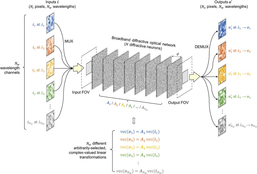
Throughout this paper, the terms “diffractive deep neural network,” “diffractive neural network,” “diffractive optical network,” and “diffractive network” are used interchangeably. Figure 1 illustrates the schematic of our broadband diffractive optical network design for massively parallel, wavelength-multiplexed all-optical computing. The broadband diffractive network, composed of eight successive diffractive layers, contains in total N diffractive neurons with their thickness values as learnable variables, which are jointly trained to perform a group of Nw linear transformations between the input and output FOVs through Nw parallel wavelength channels. More details about this diffractive architecture, its optical forward model, and training details can be found in Sec. 4. To start with, a group of Nw different wavelengths, λ1,λ2,…,λNw, are selected to be used as the wavelength channels for the broadband diffractive processor to encode different input complex fields and perform different target transformations (see Fig. 1). For the implementation of the broadband diffractive designs in this paper, we fixed the mean value λm of this group of wavelengths {λ1,λ2,…,λNw}, i.e., λm=1Nw∑w=1Nwλw and assigned these wavelengths to be equally spaced between λ1=0.9125λm and λNw=1.0875λm. Unless otherwise specified, we chose λm to be 0.8 mm in our numerical simulations, as it aligns with the terahertz band that was experimentally used in several of our previous works.50^,52^,58^,59^,61^,62^,66^,67 Without loss of generality, the wavelengths used for the design of the broadband diffractive processors can also be selected at other parts of the electromagnetic spectrum, such as the visible band, for which the related simulation results and analyses can be found in Sec. 3 to follow. Based on the scalar diffraction theory, the broadband optical fields propagating in the diffractive system are simulated at these selected wavelengths using a sampling period of 0.5λm along both the horizontal and vertical directions. We also select 0.5λm as the size of the individual neurons on the diffractive layers. With these selections, we include in our optical forward model all the propagating modes that are transmitted through the diffractive layers.

Let i and o′ be the complex-valued, vectorized versions of the 2D input and output broadband complex fields at the input and output FOVs of the diffractive network, respectively, as shown in Fig. 1. We denote iw and ow′ as the complex fields generated by sampling the optical fields at the wavelength λw(w∈{1,2,…,Nw}) within the input and output FOVs, respectively, and then vectorizing the resulting 2D matrices in column-major order. According to this notation, iw and ow′ represent the input and output of the wth wavelength channel in our wavelength-multiplexed diffractive network, respectively. In the following analyses, without loss of generality, the number of pixels at the input and output FOVs is selected to be the same, i.e., Ni=No.

To implement Nw target linear transformations, we randomly generated Nw complex-valued matrices A1,A2,…,ANw, each composed of Ni×No entries, to serve as a group of unique arbitrary linear transformations to be all-optically implemented using a wavelength-multiplexed diffractive processor. All these matrices, A1,A2,…,ANw, are generated using unique random seeds to ensure that they are different; we further confirmed the differences between these randomly generated matrices by calculating the cosine similarity values between any two combinations of the matrices in a given set (see e.g., Fig. S1 in the Supplementary Material). For each unique matrix Aw∈{A1,A2,…,ANw}, we randomly generated a total of 70,000 complex-valued input field vectors {iw} and created the corresponding output field vectors {ow} by calculating ow=Awiw. We separated these input–output complex field pairs into three individual sets for training, validation, and testing, each containing 55,000, 5000, and 10,000 samples, respectively. By increasing the size of these training data sets to >100,000 input–output pairs of randomly generated complex fields, it is possible to further improve the transformation accuracy of the trained broadband diffractive networks; since this does not change the general conclusions of this work, it is left as future work. More details on the generation of the training and testing data can be found in Sec. 4.

Based on the notations introduced above, the objective of training our wavelength-multiplexed diffractive processor is that, for any of its wavelength channels operating at λw(w∈{1,2,…,Nw}), the diffractive output fields {ow′} computed from any given inputs {iw} should provide a match to the output ground-truth (target) fields {ow}. If this can be achieved for any arbitrary choice of {iw}, this means that the all-optical transformations Aw′ performed by the trained broadband diffractive system at different wavelength channels constitute an accurate approximation to their ground-truth (target) transformation matrices Aw, where w∈{1,2,…,Nw}.

As the first step of our analysis, we selected the input/output field size to be Ni=No=8×8=64 and started to train broadband diffractive processors with Nw=2, 4, 8, 16, and 32 wavelength channels. Results and analysis of implementing more wavelength channels (e.g., Nw>100) through a single diffractive processor will be provided in later sections. For this task, we randomly generated a set of 32 different matrices with dimensions of 64×64, i.e., A1,A2,…,A32, with their first eight visualized (as examples) in Fig. 2(a) with their amplitude and phase components. Figure S1a in the Supplementary Material also reports the cosine similarity values between these randomly generated 32 matrices, confirming that they are all very close to 0. For each Nw mentioned above, we also trained several broadband diffractive designs with different numbers of trainable diffractive neurons, i.e., N ∈ {3900; 8200; 16,900; 32,800; 64,800; 131,100; 265,000}, all using the same training data sets {(iw, ow)}, randomly generated based on the target transformations {Aw} (w∈{1,2,…,Nw}) and the same number of training epochs.

To benchmark the performance of these wavelength-multiplexed diffractive networks for each N, we also trained monochromatic diffractive networks without using any wavelength multiplexing as our baseline, which can approximate only one target linear transformation using a single wavelength (i.e., Nw=1). Here we simply select λm as the operating wavelength of this baseline monochrome diffractive network used for comparison.

During the training of these diffractive networks, mean squared error (MSE) loss is calculated per wavelength channel to make the diffractive output fields come as close to the ground-truth (target) fields as possible. However, in the wavelength-multiplexed diffractive models, treating all these channels equally in the final loss function would result in the all-optical transformation accuracies being biased, since longer wavelengths present lower spatial resolution. To address this issue and equalize the all-optical transformation accuracies of all the wavelengths within the selected channel set, we devised a strategy by adaptively adjusting the weight coefficients applied to the loss terms of these channels during the training process (see Sec. 4 for details).

After the deep-learning-based training of the broadband diffractive designs introduced above is completed, the resulting all-optical diffractive transformations of these models are summarized in Figs. 2(b)–2(d). We quantified the generalization performance of these broadband diffractive networks on the blind testing data set for each transformation using three different metrics: (1) the normalized transformation MSE (MSETransformation), (2) the cosine similarity (CosSim) between the all-optical transforms and the target transforms, and (3) the MSE between the diffractive network output fields and their ground-truth output fields (MSEOutput).53^,69 More details about the definitions of these performance metrics are provided in Sec. 4. For the diffractive designs with different numbers of wavelength channels (Nw=1, 2, 4, 8, 16, and 32), we report these performance metrics in Figs. 2(b)–2(d) as a function of the number of trainable diffractive neurons (N). These performance metrics reported in Fig. 2 refer to the mean values calculated across all the wavelength channels, whereas the results of the individual wavelength channels are shown in Fig. 3.

In Fig. 2(b), it can be seen that the transformation errors of all the trained diffractive models show a monotonic decrease as N increases, which is expected due to the increased degrees of freedom in the diffractive processor. Also the approximation errors of the regular diffractive networks without using wavelength multiplexing, i.e., Nw=1, approaches 0 as N approaches 2NiNo≈8200. This observation confirms the conclusion obtained in our previous work,69^,70 i.e., a phase-only monochrome diffractive network requires at least 2NiNo diffractive neurons to approximate a target complex-valued linear transformation with negligible error. On the other hand, for the wavelength-multiplexed diffractive models with Nw different wavelength channels that are trained to approximate Nw unique linear transforms, we see in Fig. 2 that the approximation errors approach 0 as N approaches 2NwNiNo. This finding indicates that compared to a baseline monochrome diffractive model that can only perform a single transform, performing multiple distinct transforms using wavelength multiplexing within a single diffractive network requires its number of trainable neurons N to be increased by Nw-fold. This conclusion is further supported by the results of the other two performance metrics, CosSim and MSEOutput, as shown in Figs. 2(c) and 2(d): as N approaches 2NwNiNo, CosSim and MSEOutput of the wavelength-multiplexed diffractive models approach 1 and 0, respectively.

To reveal the linear transformation performance of the individual wavelength channels in our wavelength-multiplexed diffractive processors, in Fig. 3, we show the channel-wise output field errors (MSEOutput) of the wavelength-multiplexed diffractive networks with Nw=2, 4, 8, 16, and 32 and N=2NwNiNo. Figure 3 indicates that the MSEOutput of these individual channels are very close to each other in all the designs with different Nw, demonstrating no significant performance bias toward any specific wavelength channel or target transform. For comparison, we also show in Fig. S2 in the Supplementary Material, the resulting MSEOutput of the diffractive model with Nw=8 and N=2NwNiNo=16NiNo when our channel balancing training strategy with adaptive weights was not used (see Sec. 4). There appears to be a large variation at the output field errors among the different wavelength channels if adaptive weights were not used during the training; in fact, the channels assigned to longer wavelengths tend to show much inferior transformation performance, which highlights the significance of using our balancing strategy during the training process. Stated differently, unless a channel balancing strategy is employed during the training phase, longer wavelengths suffer from relatively lower spatial resolution and face increased all-optical transformation errors compared to the shorter wavelength channels.

To visually demonstrate the success of our broadband diffractive system in performing a group of linear transformations using wavelength multiplexing, in Fig. 4, we show examples of the ground-truth transformation matrices (i.e., Aw) and their all-optical counterparts (i.e., Aw′) resulting from the diffractive designs with Nw=8 and N∈{2NwNiNo=16NiNo=64,800;4NwNiNo=32NiNo=131,100}. The amplitude and phase absolute errors between the two (Aw and Aw′) are also reported in the same figure. Moreover, in Fig. 5 and Fig. S3 in the Supplementary Material, we present some exemplary complex-valued input–output optical fields from the same set of diffractive designs with N=4NwNiNo=131,100 and N=2NwNiNo=64,800, respectively. These results, summarized in Figs. 4 and 5 and Fig. S3 in the Supplementary Material, reveal that, when N≥2NwNiNo, the all-optical transformation matrices and the output complex fields of all the wavelength channels match their ground-truth targets very well with negligible error, which is also in line with our earlier observations in Fig. 2.

We have so far demonstrated that a single broadband diffractive network can be designed to simultaneously perform a group of Nw arbitrary complex-valued linear transformations, with Nw=2, 4, 8, 16, and 32 (Figs. 2 and 3). Next, we explore the feasibility of implementing a significantly larger number of wavelength channels in our system to better understand the limits of Nw. Due to our limited computational resources available, to simulate the behavior of larger Nw values, we selected Ni=No=5×5 and Nw∈{1,2,4,8,16,32,64,128,and184}. Accordingly, we generated a new set of 184 different arbitrarily selected complex-valued matrices with dimensions of 25×25, i.e., A1,A2,…,A184, as the target linear transformations to be all-optically implemented. The cosine similarity values between these randomly generated matrices are reported in Fig. S1b in the Supplementary Material, confirming that they are all very close to 0. We also created training, validation, and testing data sets based on these new target transformation matrices following the same approach as in the previous section: for each transformation matrix, we randomly generated 55,000, 5000, and 10,000 field samples for the training, validation, and testing data sets, respectively. Then using the training field data sets, we trained broadband diffractive designs with Nw different wavelength channels, where the Nw target transforms were taken from the first Nw matrices in the randomly generated set {A1,A2,…,A184}. For each Nw choice, we also trained diffractive models with different numbers of diffractive neurons, including N=1.5NwNiNo, N=2NwNiNo, and N=3NwNiNo.

The all-optical transformation performance metrics of the resulting diffractive networks on the testing data sets are shown in Fig. 6 as a function of Nw. Figures 6(a)–6(c) reveal that the all-optical transformations of the diffractive designs with different N show some increased error as Nw increases. For the diffractive models with N=3NwNiNo, the all-optical transformation errors (MSETransformation) at smaller Nw appear to be extremely small and do not exhibit the same performance degradation with increasing Nw; only after Nw>10 we see an error increase in the all-optical transformations for N=3NwNiNo. By comparing the linear transformation performance of the models with different N, Fig. 6 clearly reveals that adding more diffractive neurons to a broadband diffractive network design can greatly improve its transformation performance, which is especially important to operate at a large Nw.

By having a linear fit to the data points shown in Figs. 6(a) and 6(c), we can extrapolate to larger Nw values and predict an all-optical transformation error bound as a function of Nw. With these fitted (dashed) lines shown in Figs. 6(a) and 6(c), we get a coarse prediction of the linear transformation performance of a broadband diffractive model with a significantly larger number of wavelength channels Nw that is challenging to simulate due to our limited computer memory and speed. Interestingly, these three fitted lines (corresponding to diffractive designs with N=1.5NwNiNo, N=2NwNiNo, and N=3NwNiNo) intersect with each other at a point around Nw=10,000 with an MSETransformation of ∼0.2 and an MSEOutput of ∼0.03. This level of transformation error coincides with the error levels observed at the beginning of our training, implying that a broadband diffractive model with Nw=∼10,000, even after training, would only exhibit a performance level comparable to an untrained model. These analyses indicate that, for a broadband diffractive network trained with N≤3NwNiNo and a training data set of 55,000 optical field pairs, there is an empirical multiplexing upper bound of Nw=∼10,000.

However, before reaching this Nw=∼10,000 ultimate limit discussed above, practically the desired level of approximation accuracy will set the actual limit of Nw. For example, based on visual inspection and the calculated peak signal-to-noise ratio (PSNR) values, one can empirically choose a blind testing error of MSEOutput∼10−3 as a threshold for the diffractive network’s all-optical approximation error; this threshold corresponds to a mean PSNR value of ∼20dB, calculated for the diffractive network output fields against their ground truth (see Fig. S4 in the Supplementary Material). We marked this MSEOutput-based performance threshold in Fig. 6(c) using a black dashed line, which also corresponds to a transformation error (MSETransformation) of ∼9×10−3, which was also marked in Fig. 6(a) with a black dashed line. Based on these empirical performance thresholds set by MSEOutput≈10−3 and PSNR≈20dB, we can infer that a broadband diffractive processor with N=3NwNiNo can accommodate up to Nw∼2000 wavelength channels, where ∼2000 different linear transformations can be performed through a single broadband diffractive processor within the performance bounds shown in Figs. 6(a) and 6(c) (see the purple dashed lines). The same analysis reveals a reduced upper bound of Nw∼600 for the diffractive network designs with N=2NwNiNo (see the green dashed lines).

In the previous section, we showed that a broadband diffractive processor can be designed to implement >180 different target linear transforms simultaneously, and this number can be further extended to Nw∼2000 based on an all-optical approximation error threshold of MSEOutput≈10−3. In this section, we provide additional analyses on material-related factors that have an impact on the accuracy of wavelength-multiplexed computing through broadband diffractive networks. For example, the selection of materials with different dispersion properties (i.e., the real and imaginary parts of the refractive index as a function of the wavelength) will impact the light–matter interactions at different illumination wavelengths. To numerically explore the impact of material dispersion and related optical losses, we took the broadband diffractive network design shown in Fig. 6 with Nw=128 and N=3NwNiNo and retrained it using different materials. The first material we selected is a lossy polymer that is widely employed as a 3D printing material; this material was used to fabricate diffractive networks that operate at the terahertz part of the spectrum.52^,66^,67 The dispersion curves of this lossy material are shown in Fig. S5a in the Supplementary Material, which were also used in the design of the diffractive networks reported in the previous sections (with λm=0.8mm). As a second material choice for comparison, we selected a lossless dielectric material, for which we took N-BK7 glass as an example and used its dispersion to simulate our wavelength-multiplexed diffractive processor design at the visible wavelengths with λm=530nm; the dispersion curves of this material are reported in Fig. S5b in the Supplementary Material. As a third material choice for comparison, we considered a hypothetical scenario where the material of the diffractive layers had a flat dispersion at around λm=0.8mm, with no absorption and a constant refractive index (∼1.72) across all the selected wavelength channels of interest; see the refractive index curve of this “dispersion-free” material in Fig. S5c in the Supplementary Material.

After the training of the diffractive network models using these different materials selected for comparison, we summarized their all-optical linear transformation performance in Figs. 7(a)–7(c) (see the purple bars). These results reveal that all three diffractive models with different material choices achieved negligible all-optical transformation errors, regardless of their dispersion characteristics. This confirms the feasibility of extending our wavelength-multiplexed diffractive processor designs to other spectral bands with vastly different material dispersion features.

In addition to the all-optical transformation accuracy, the output diffractive efficiency (η) of these diffractive network models is also practically important. As shown in Fig. 7(d), due to the absorption by the layers, the diffractive network model using the lossy polymer material presents a very poor output diffraction efficiency η compared to the other two diffractive models that used lossless materials. In addition to the absorption of light through the diffractive layers, a wavelength-multiplexed diffractive network also suffers from optical losses due to the propagating waves that leak out of the diffractive processor volume. This second source of optical loss within a diffractive network can be strongly mitigated through the incorporation of diffraction efficiency-related penalty terms52^,66^,67^,69 into the training loss function (see Sec. 4 for details). The results of using such a diffraction-efficiency-related penalty term during training are presented in Figs. 7(a)–7(d) (yellow bars), which indicate that the output diffraction efficiencies of the corresponding models were improved by >589 to 1479-fold compared to their counterparts that were trained without using such a penalty term [see Fig. 7(d)]. We also show in Figs. 7(e) and 7(f), the output diffraction efficiencies of the individual wavelength channels trained without and with the diffraction-efficiency penalty term, respectively. These results also revealed that the diffraction-efficiency-related penalty term used during training not only improved the overall output efficiency of the diffractive processor design but also helped to mitigate the imbalance of diffraction efficiencies among different wavelength channels [see Figs. 7(e) and 7(f)]. These improvements also come at an expense; as shown in Figs. 7(a)–7(c), there is some degradation in the all-optical transformation performance of the diffractive networks that are trained with a diffraction-efficiency-related penalty term. However, this relative degradation in the all-optical transformation performance is still acceptable, since a cosine similarity value of >0.996 to 0.998 is maintained in each case [see Fig. 7(b), yellow bars].

The bit depth of a broadband diffractive network refers to the finite number of thickness levels that each diffractive neuron can have on top of a common base thickness of each diffractive layer. For example, in a broadband diffractive network with a bit depth of 8, its diffractive neurons will be trained to have at most 28=256 different thickness values that are distributed between a predetermined minimum thickness and a maximum thickness value. To mechanically support each diffractive layer, the minimum thickness is always positive, acting as the base thickness of each layer. To analyze the impact of this bit depth on the linear transformation performance and accuracy of our wavelength-multiplexed diffractive networks, we took the Nw=184 channel diffractive design reported in the previous sections (trained using a data format with 32-bit depth) and retrained it from scratch under different bit depths, including 4, 8, and 12. Based on the same test data set, the all-optical linear transformation performance metrics of the resulting diffractive networks are reported in Fig. 8 as a function of N. Figure 8 reveals that a 12-bit depth is practically identical to using a 32-bit depth in terms of the all-optical transformation accuracy that can be achieved for the Nw=184 target linear transformations. Furthermore, a bit depth of 8 can also be used for a broadband diffractive network design to maintain its all-optical transformation performance with a relatively small error increase, which can be compensated for with an increase in N, as illustrated in Fig. 8. These observations from Fig. 8 highlight (1) the importance of having a sufficient bit depth in the design and fabrication of a broadband diffractive processor and (2) the importance of N as a way to boost the all-optical transformation performance under a limited diffractive neuron bit depth.

Another possible factor that may cause systematic errors in our framework is the wavelength precision or jitter. To analyze the wavelength encoding related errors, we used the four-channel wavelength-multiplexed diffractive network model with N≈2NwNiNo=8NiNo and Ni=No=82 that was presented in Fig. 3(b). We deliberately shifted the illumination wavelength used for each encoding channel away from the preselected wavelength used during the training (i.e., λ1=0.9125λm, λ2=0.9708λm, λ3=1.0292λm, and λ4=1.0875λm). The resulting linear transformation performance of the Nw=4 channels using different performance metrics is summarized in Figs. 9(a)–9(c) as a function of the illumination wavelength. All of these results in Fig. 9 show that as the illumination wavelengths used for each encoding channel gradually deviate from their designed/assigned wavelengths (used during the training of the wavelength-multiplexed diffractive network), their all-optical transformation accuracy begins to degrade. To shed more light on this, we used the previous performance threshold based on MSEOutput≈10−3 as an empirical criterion to estimate the tolerable range of illumination wavelength errors, which revealed an acceptable bandwidth of ∼0.002λm for each one of the encoding wavelength channels. Stated differently, when a given illumination wavelength is within ±∼0.001λm of the corresponding preselected wavelength assigned for that spectral channel, the degradation of the linear transformation accuracy at the output of the wavelength-multiplexed diffractive network will satisfy MSEOutput≤10−3. In practical applications, this level of spectral precision can be routinely achieved by using high-performance wavelength scanning sources74^,75 (e.g., swept-source lasers) or narrow passband thin-film filters.

So far, we have demonstrated the design of wavelength-multiplexed diffractive processors that can allow a massive number of unique complex-valued linear transformations to be computed, all in parallel, within a single diffractive optical network. To exemplify some of the potential applications of this broadband diffractive processor design, here we demonstrate the permutation matrix-based optical transforms, which have significance for telecommunications (e.g., channel routing and interconnects), information security, and data processing (see Fig. 10). Similar to the approaches introduced earlier, we randomly generated eight permutation matrices, P1,P2,…,P8 [see Fig. 10(b)] and trained a wavelength-multiplexed diffractive network with Nw=8 and N=2NwNiNo=16NiNo=64,800; this architecture has the same configuration as the one shown in Fig. 3(c), and Fig. 4 (middle column), except it uses these new permutation matrices as the target transforms. After its training, in Fig. 10(a), we show examples of permutation-based encoding of input images using the trained broadband diffractive network. After being all-optically processed by our wavelength-multiplexed diffractive network design, all the input images (iw) are simultaneously permuted (encoded) according to the permutation matrices assigned to the corresponding wavelength channels, resulting in the output fields ow′, which very well match their ground truth ow [see Fig. 10(a)]. Stated differently, the trained wavelength-multiplexed diffractive processor can successfully synthesize the correct output field ow=Pwiw for all the possible input fields iw, since it presents an all-optical approximation of Pw for w∈{1,2,…,8}.

Similarly, we present in Fig. S6 in the Supplementary Material that the same wavelength-multiplexed permutation transformation network can be used to all-optically decode the encoded/permuted patterns. In this case, the input encoded fields are generated by transforming (permuting) the same input images using the inverse of the permutation matrices P1,P2,…,P8. The results shown in Fig. S6 in the Supplementary Material indicate that the wavelength-multiplexed diffractive network can all-optically perform simultaneous decoding of all the input images, very well matching their ground truth.

Next, we performed a proof-of-concept experimental validation of our diffractive network using wavelength-multiplexed permutation operations. With a frequency-tunable continuous-wave terahertz (THz) setup shown in Fig. 11(a) (see Sec. 4 for its implementation details), we tested a wavelength-multiplexed diffractive network design with Nw=2 and Ni=No=32, where the two wavelength channels were chosen as λ1=0.667mm and λ2=0.698mm. Each one of these two wavelength channels in this experimental design is assigned to a unique, arbitrarily generated target permutation matrix (P1 and P2, see Fig. S7 in the Supplementary Material), such that any spatially structured pattern at the input FOV can be all-optically permuted by the diffractive optical network to form different desired patterns at the output FOV, performing P1 and P2 under λ1 and λ2 illumination, respectively. For this, we used a diffractive network architecture with three diffractive layers, with each layer having 120×120 diffractive features, each with a lateral size of 0.4 mm (∼0.59λm). The axial spacing between any two of the adjacent layers (including the input/output planes) in this design was set as 20 mm (∼29.3λm). During the training process, a total of 55,000 randomly generated input–output field pairs corresponding to the target permutation matrices (P1 and P2) were used to update the thickness values of these diffractive layers. After the training converged, the resulting diffractive layers were fabricated using a 3D printer and mechanically assembled to form a physical wavelength-multiplexed diffractive optical permutation processor, as shown in Figs. 11(b)–11(d).

To experimentally test the performance of this 3D-fabricated wavelength-multiplexed diffractive network, different input patterns from the blind testing set (never used in training) were also 3D-printed and used as the input test objects. The experimental test results are reported in Fig. 11(e), revealing that the output patterns for all these input patterns show a good agreement with their numerically simulated counterparts and the ground-truth images. The success of these experimental results further confirms the feasibility of our wavelength-multiplexed diffractive optical transformation networks.

We demonstrated wavelength-multiplexed diffractive network designs that can perform massively parallel universal linear transformations through a single diffractive processor. We also quantified the limits of Nw and the impact of material dispersion, bit depth, and wavelength precision/jitter on the all-optical transformation performance of broadband diffractive networks. In addition to these, other factors may limit the performance of broadband diffractive processors, including the lateral and axial misalignments of diffractive layers, surface reflections, and other imperfections introduced during the fabrication. To mitigate some of these practical issues, various approaches, such as high-precision lithography and antireflection coatings can be utilized in the fabrication process of a diffractive network. As demonstrated in our previous work,50^,52^,61 it is also possible to mitigate the performance degradation resulting from some of these experimental factors by incorporating them as random errors into the physical forward model used during the training process, which is referred to as “vaccination” of the diffractive network.

The reported wavelength-multiplexed diffractive processor represents a milestone in expanding the parallelism of diffractive all-optical computing, simultaneously covering a large group of complex-valued linear transformations. Compared to our previous work,70 where a monochromatic diffractive optical network was integrated with polarization-sensitive elements to achieve multiplexing of four independent linear transformations, the multiplexing factor (Nw) of a wavelength-multiplexed diffractive network is significantly increased to more than 180, and can further reach Nw∼2000, revealing a major improvement in the all-optical processing throughput. Moreover, the physical architecture of this wavelength-multiplexed computing framework is also relatively simple, since it does not rely on any additional optical modulation elements, e.g., spectral filters; it solely utilizes the different phase modulation values of the same diffractive layers at different wavelengths of light, also being compatible with different materials with various dispersion properties (including flat dispersion, as illustrated in Fig. 7). One could perhaps argue that, equivalent to a wavelength-multiplexed diffractive network that uses N trainable diffractive features to compute Nw independent target linear transformations, we could utilize a set of Nw separately optimized monochromatic diffractive networks, each assigned to perform one of the Nw target linear transforms using N/Nw diffractive features. However, such a multipath design involving Nw different monochromatic diffractive networks (one for each target transformation) would require bulky optical routing for fan-in/fan-out, which would introduce additional insertion losses, noise, and misalignment errors into the system, thus hurting the energy efficiency, performance, and compactness of the optical processor. Considering the fact that we covered Nw>180 in this work, such an approach of using Nw separate monochromatic diffractive networks is not a feasible strategy that can compete with a wavelength-multiplexed design. Furthermore, if additional multiplexing schemes other than the wavelength multiplexing reported here were to be used, such as temporal multiplexing, switching between different diffractive networks, they would also require the use of additional optoelectronic control elements, further increasing the hardware complexity of the system, which would not be feasible for a large Nw.

It is worth further emphasizing that even if multiple separately optimized monochromatic diffractive networks could be trained to individually perform different target linear transforms at different wavelengths, it is not possible to directly combine the converged/optimized layers of these diffractive networks to match the broadband operation of the wavelength-multiplexed diffractive network presented here. Since these monochromatic networks are individually trained using only a single illumination wavelength, the optimized modulation of each wavelength under broadband illumination would produce destructive patterns to other wavelengths, and their transformation accuracies would be collectively hampered. This, once again, highlights the significance of our wavelength multiplexing scheme: a wavelength-multiplexed diffractive optical network can be realized through the engineering of the surface profiles of dielectric diffractive layers with arbitrary dispersion properties, whereas these profiles should be designed by simultaneously taking into account all the Nw wavelength channels, with phase modulation values that are mutually coupled to each other.

To the best of our knowledge, there has not been a demonstration of a design for the all-optical implementation of a complex-valued, arbitrary linear transformation using metasurfaces or metamaterials. In principle, having different diffractive metaunits placed on the same substrate to perform different transformations at different wavelengths could be attempted as an alternative approach to what we presented in this paper. However, such an approach would face severe challenges since (1) at large spectral multiplexing factors (Nw≫1) shown in this work, the lateral period for each spectral metadesign will substantially increase per substrate, lowering the accuracy of each transformation; (2) at each illumination wavelength, the other metaunits designed for (assigned to) the other spectral components, will also introduce “cross-talk fields” that will severely contaminate the desired responses at each wavelength and cannot be neglected since Nw≫1; (3) the phase responses of the spectrally encoded metaunits, in general, cover a small angular range, leading to low numerical aperture (NA) solutions compared to the diffractive solutions reported in this work, where NA = 1 (in air); the low NA of metaunits fundamentally limits the space-bandwidth product of each transformation channel; and (4) if multiple layers of metasurfaces are used in a given design, all of these aforementioned sources of errors associated with spectral metaunits will accumulate and get amplified through the subsequent field propagation in a cascaded manner, causing severe degradations to the final output fields, compared to the desired fields. Perhaps due to these significant challenges outlined here, metasurface or metamaterial-based diffractive designs have not yet been reported as a solution to perform universal linear transformations—neither an arbitrary complex-valued linear transformation nor a group of linear transformations through some form of multiplexing.

As we have shown in Sec. 2, a diffractive neuron number of N≥2NwNiNo is required for a wavelength-multiplexed diffractive network to successfully implement Nw different complex-valued linear transforms. Compared to the previous complex-valued monochrome (Nw=1) diffractive designs,69 the additional factor of 2 in N results from the fact that the only trainable degrees of freedom for a broadband wavelength-multiplexed diffractive design are the thickness values of the diffractive neurons, whereas the Nw different target transformations are all complex-valued. Stated differently, the resulting modulation values of different wavelengths through each diffractive neuron are mutually coupled through the dispersion of the material and depend on the neuron thickness.

Finally, we would like to emphasize that this presented framework can operate at various parts of the electromagnetic spectrum, including the visible band, so that the set of wavelength channels used to perform the transformation multiplexing can match with the light source and/or the spectral signals emitted from or reflected by the objects. In practice, this massively parallel linear transformation capability can be utilized in an optical processor to perform distinct statistical inference tasks using different wavelength channels, bringing in additional throughput and parallelism to optical computing. This wavelength-multiplexed diffractive network design might also inspire the development of new multicolor and hyperspectral machine-vision systems, where all-optical information processing is performed simultaneously based on both the spatial and spectral features of the input objects. The resulting hyperspectral or multispectral diffractive output fields can enable new optical visual processing systems that can identify or encode input objects with unique spectral properties. As another possibility, novel multispectral display systems can be created using these wavelength-multiplexed diffractive output fields to reconstruct spectroscopic images or light fields from compressed or distorted input spectral signals.62 All these possibilities enabled by wavelength-multiplexed diffractive optical processors can inspire numerous applications in biomedical imaging, remote sensing, analytical chemistry, material science, and many other fields.

A wavelength-multiplexed diffractive network consists of successive diffractive layers that collectively modulate the incoming broadband optical fields. In the forward model of our numerical simulations, the diffractive layers are assumed to be thin optical modulation elements, where the mth feature on the kth layer at a spatial location (xm,ym,zm) represents a wavelength-dependent complex-valued transmission coefficient tk given by tk(xm,ym,zm,λ)=ak(xm,ym,zm,λ)exp(jϕk(xm,ym,zm,λ)),(1)where a and ϕ denote the amplitude and phase coefficients, respectively. The diffractive layers are connected to each other by free-space propagation, which is modeled through the Rayleigh–Sommerfeld diffraction equation:22^,46fmk(x,y,z)=z−zir2(12πr+1jλ)exp(j2πrλ),(2)where fmk(x,y,z,λ) is the complex-valued field on the mth pixel of the kth layer at (x,y,z) at a wavelength of λ, which can be viewed as a secondary wave generated from the source at (xm,ym,zm); and r=(x−xm)2+(y−ym)2+(z−zm)2 and j=−1. For the kth layer (k≥1, assuming the input plane is the 0th layer), the modulated optical field Ek at location (xm,ym,zm) is given by Ek(xm,ym,zm,λ)=tk(xm,ym,zm)·∑n∈SEk−1(xn,yn,zn,λ)·fmk−1(xm,ym,zm),(3)where S denotes all the diffractive neurons on the previous diffractive layer.

For the diffractive models used for numerical analyses, we chose λm/2 as the smallest sampling period for the simulation of the complex optical fields and also used λm/2 as the smallest feature size of the diffractive layers. In the input and output FOVs, a 4×4 binning is performed on the simulated optical fields, resulting in a pixel size of 2λm for the input/output fields. The axial distance (d) between the successive layers (including the diffractive layers and the input/output planes) in our diffractive processor designs is empirically selected as d=0.5Dlayer, where Dlayer represents the lateral size of each diffractive layer.

The diffractive thickness value h of each neuron of a diffractive layer is composed of two parts hlearnable and hbase as follows: h=hlearnable+hbase,(4)where hlearnable denotes the learnable thickness parameters of each diffractive feature and is confined between hmin=0 and hmax=1.25λm for all the diffractive models used for numerical analyses in this paper. When a modulation with q-bit depth is applied to the diffractive model, hlearnable will be rounded to the nearest number that corresponds to one of 2q different equally spaced levels within the range of [0, hlearnable]. The additional base thickness hbase is a constant, which is chosen as 0.25λm to serve as substrate support for the diffractive neurons. To achieve the constraint applied to hlearnable, an associated latent trainable variable hv was defined using the following analytical form: hlearnable=hmax2·(sin(hv)+1).(5)

Note that before the training starts hv values of all the diffractive neurons were randomly initialized with a normal distribution (a mean value of 0 and a standard deviation of 1). Based on these definitions, the amplitude and phase components of the complex transmittance of mth, i.e., ak(xm,ym,zm,λ) and ϕk(xm,ym,zm,λ), can be written as a function of the thickness of each neuron hm and the incident wavelength λ: ak(xm,ym,zm,λ)=exp(−2πκ(λ)hmkλ),(6)ϕk(xm,ym,zm,λ)=(n(λ)−nair)2πhmkλ,(7)where the wavelength-dependent parameters n(λ) and κ(λ) are the refractive index and the extinction coefficient of the diffractive layer material corresponding to the real and imaginary parts of the complex-valued refractive index n˜(λ), i.e., n˜(λ)=n(λ)+jκ(λ).66 In the numerical analyses of this work, we considered three different materials to form the diffractive layers of a broadband diffractive processor, including a lossy polymer, a lossless dielectric, and a hypothetical lossless dispersion-free material. Among these, the lossy polymer material represents a UV-curable 3D printing material (VeroBlackPlus RGD875, Stratasys Ltd.), which was used in our previous work52^,66^,67 for 3D printing of diffractive networks. The lossless dielectric material, used for the diffractive models operating at the visible band, represents N-BK7 glass (Schott), ignoring the negligible absorption through thin layers. The dispersion-free material, on the other hand, assumed a lossless material with its refractive index n(λ) having a flat distribution with respect to the wavelength range of interest, i.e., n(λ)≈1.72. The final n(λ) and κ(λ) curves of different materials that were used for training the diffractive models reported in this paper are shown in Fig. S5 in the Supplementary Material.

In this paper, the input and output FOVs of the diffractive networks are assumed to have the same size, which is set as 8×8, 5×5, or 3×3pixels based on the assigned linear transformation tasks, i.e., iw,ow∈C8×8, C5×5, or C3×3 (w∈{1,2,…,Nw}). Accordingly, the size of the target complex-valued transformation matrices Aw is equal to 64×64, 25×25, or 9×9, respectively, i.e., Aw∈C64×64 (w∈{1,2,…,32}), Aw∈C25×25(w∈{1,2,…,184}), or Aw∈C9×9 (w∈{1,2}). For arbitrary linear transformations, the amplitude and phase components of all these target matrices Aw were generated with a uniform (U) distribution of U[0,1] and U[0,2π], respectively, using the pseudorandom number generation function random.uniform() built-in NumPy. For the arbitrarily selected permutation transformations, all the target matrices Aw (also denoted as Pw) were generated by permuting an identity matrix of the same size as Pw using the pseudorandom matrix permutation function random.permutation() built-in NumPy. Different random seeds were used to generate these transformation matrices to ensure they were unique. For training a broadband diffractive network with Nw wavelength channels, the amplitude and phase components of the input fields iw (w∈{1,2,…,Nw}) were randomly generated with a uniform (U) distribution of U[0,1] and U[0,2π], respectively. The ground-truth (target) fields ow (w∈{1,2,…,Nw}) were generated by calculating ow=Awiw. For each Aw (w∈{1,2,…,Nw}), we generated a total of 70,000 input/output complex optical fields to form a data set, which was then divided into three parts: training, validation, and testing, each containing 55,000, 5000, and 10,000 complex-valued optical field pairs, respectively.

For each wavelength channel, the normalized MSE loss function is defined as $$\begin{gathered} LMSE,w=E[1No∑n=1No|ow^[n]−ow′^[n]|2] \\ =E[1No∑n=1No|σwow[n]−σw′ow′[n]|2], \end{gathered}$$(8)where E[·] denotes the average across the current batch, w stands for the wth wavelength channel that is being accessed, and [n] indicates the nth element of the vector. σw and σw′ are the coefficients used to normalize the energy of the ground-truth (target) field ow and the diffractive network output field ow′, respectively, which are given by σw=1∑n=1No|ow[n]|2,(9)σw′=∑n=1Noσwow[n]ow′*[n]∑n=1No|ow′[n]|2.(10)

During the training of each broadband diffractive network, all the wavelength channels are simultaneously simulated, and the training data are fed into the channels at the same time. The wavelength-multiplexed diffractive network is trained based on the loss averaged across different wavelength channels. The total loss function L that we used can be written as L=1Nw∑w=1NwαwLMSE,w,(11)where αw is the adaptive spectral weight coefficient applied to the loss for the wth wavelength channel, which was used to balance the performance achieved by different wavelength channels during the optimization process. The initial values of αw for all the wavelength channels are set as 1. After the optimization begins, αw is adaptively updated after each training step using the following equation: αw←max(0.1×(LMSE,w−LMSE,wref)+αw,0),(12)where LMSE,wref represents the MSE loss of the wavelength channel that is chosen to be a reference to measure the difference in the loss of the other channels. This also means that αw for the wavelength channel selected as the reference remains unchanged at 1. For the trained broadband diffractive models presented in this paper, we chose the middle channel as the reference wavelength channel, i.e., wref=Nw/2. According to this approach, for a wavelength channel w that is not a reference channel, when the loss of the channel is small compared to that of the reference channel, αw will automatically decrease to reduce the weight of the corresponding channel. Conversely, when the loss of a specific wavelength channel is large compared to that of the reference channel, αw will automatically grow to increase the weight of the channel and thus enhance the subsequent penalty on the corresponding channel performance.

In order to increase the output diffraction efficiencies of the diffractive networks, we incorporated an additional efficiency penalty term to the loss function of Eq. (11): L=1Nw∑w=1Nw(αwLMSE,w+βLeff,w),(13)where Leff,w represents the diffraction efficiency penalty loss applied to the wth wavelength channel, and β represents its weight, empirically set as 104. Leff,w is defined as Leff,w={ηth−ηw,ifηth≥ηw0,ifηth<ηw,(14)where ηw represents the mean output diffraction efficiency for the wth wavelength channel of the wavelength-multiplexed diffractive network, and ηth refers to a predetermined penalization threshold, which was taken as 3×10−5 (for diffractive models using the lossy polymer materials) or 3×10−4 (for the other diffractive models using lossless dielectric or dispersion-free materials). ηw is defined as ηw=E[∑n=1No|ow′[n]|2∑n=1Ni|iw[n]|2].(15)

To quantitatively evaluate the transformation results of the wavelength-multiplexed diffractive networks, four different performance metrics were calculated per wavelength channel of the diffractive designs using the blind testing data set: (1) the normalized transformation MSE (MSETransformation), (2) the cosine similarity (CosSim) between the all-optical transforms and the target transforms, (3) the normalized MSE between the diffractive network output fields and their ground truth (MSEOutput), and (4) the output diffraction efficiency [Eq. (15)]. The transformation error for the wth wavelength channel of the wavelength-multiplexed diffractive network MSETransformation,w is defined as $$\begin{gathered} MSETransformation,w=1NiNo∑n=1NiNo|aw[n]−mwaw′[n]|2 \\ =1NiNo∑n=1NiNo|aw[n]−aw′^[n]|2, \end{gathered}$$(16)where aw is the vectorized version of the ground-truth (target) transformation matrix assigned to the wth wavelength channel Aw, i.e., aw=vec(Aw). aw′ is the vectorized version of Aw′, which is the all-optical transformation matrix performed by the trained diffractive network. mw is a scalar coefficient used to eliminate the effect of diffraction efficiency-related scaling mismatch between Aw and Aw′, i.e., mw=∑n=1NiNoaw[n]aw′*[n]∑n=1NiNo|aw′[n]|2.(17)

The cosine similarity between the all-optical diffractive transform and its target (ground truth) for the wth wavelength channel CosSimw is defined as CosSimw=|awHa^w′|∑n=1NiNo|aw[n]|2∑n=1NiNo|aw′^[n]|2.(18)

The normalized MSE between the diffractive network outputs and their ground truth for the wth wavelength channel MSEOutput,w is defined using the same formula as in Eq. (8), except that E[·] is calculated across the entire testing set.

All the diffractive optical networks used in this work were trained using PyTorch (v1.11.0, Meta Platforms Inc.). We selected AdamW optimizer76^,77 for training all the models, and its parameters were taken as the default values and kept identical in each model. The batch size was set as 8. The learning rate, starting from an initial value of 0.001, was set to decay at a rate of 0.5 every 10 epochs, respectively. The training of the diffractive network models was performed with 50 epochs. The best models were selected based on the MSE loss calculated on the validation data set. For the training of our diffractive models, we used a workstation with a GeForce RTX 3090 graphical processing unit (Nvidia Inc.) and Intel^® Core™ i9-12900F central processing unit (Intel Inc.) and 64 GB of RAM, running Windows 11 operating system (Microsoft Inc.). The typical time required for training a wavelength-multiplexed diffractive network model with, e.g., Nw=128 and N=1.5NwNiNo is ∼50h.

The diffractive layers used in our experiments were fabricated using a 3D printer (PR110, CADworks3D). The input test objects and holders were also 3D-printed (Objet30 Pro, Stratasys). After the printing process, the input objects were coated with aluminum foil to define the light-blocking areas, leaving openings at specific positions to define the transmitted pixels of the input patterns. The designed holder was used to assemble the diffractive layers and objects to mechanically maintain their relative spatial positions in line with our numerical design.

To test our fabricated wavelength-multiplexed diffractive network design, we adopted a THz continuous-wave scanning system, whose schematic is presented in Fig. 11(a). A WR2.2 modular amplifier/multiplier chain (AMC) followed by a compatible diagonal horn antenna (Virginia Diode Inc.) is used as the THz source. Each time, a 10-dBm RF input signal was set at 11.944 or 12.500 GHz (fRF1) at the input of AMC and multiplied 36 times to generate output radiation at 450 or 430 GHz, respectively, which corresponds to the illumination wavelengths λ1=0.667mm and λ2=0.698mm used for the two wavelength channels. A 1-kHz square wave was also generated to modulate the AMC output for lock-in detection. By placing the wavelength-multiplexed diffractive network 600 mm away from the exit aperture of the THz source, an approximately uniform plane wave was created, impinging on the input FOV of the diffractive network. The intensity distribution within the output FOV of the diffractive network was scanned at a step size of 2 mm by a single-pixel mixer/AMC (Virginia Diode Inc.) detector, which was mounted on an XY positioning stage formed by combining two linearly motorized stages (Thorlabs NRT100). For illumination at λ1=0.667mm or λ2=0.698mm, a 10-dBm sinusoidal signal was also generated at 11.917 or 12.472 GHz (fRF2), respectively, as a local oscillator and sent to the detector to downconvert the output signal to 1 GHz. After being amplified by a low-noise amplifier (Mini-Circuits ZRL-1150-LN+) with a gain of 80 dBm, the downconverted signal was filtered by a 1-GHz (±10MHz) bandpass filter (KL Electronics 3C40-1000/T10-O/O) and attenuated by a tunable attenuator (HP 8495B) for linear calibration. This final signal was then measured by a low-noise power detector (Mini-Circuits ZX47-60), whose output voltage was read by a lock-in amplifier (Stanford Research SR830) using the 1-kHz square wave as the reference signal and calibrated to a linear scale. In our postprocessing, cropping and pixel binning were applied to each measurement of the intensity field to match the pixel size and position of the output FOV used in the design phase, resulting in the output measurement images shown in Fig. 11(e).

Jingxi Li received his BS degree in optoelectronic information science and engineering from Zhejiang University, Hangzhou, Zhejiang, China, in 2018. Currently, he is working toward his PhD in the Electrical and Computer Engineering Department, University of California, Los Angeles, California, United States. His work focuses on optical computing and information processing using diffractive networks and computational optical imaging for biomedical applications.

Tianyi Gan received his BS degree in physics from Peking University, Beijing, China, in 2021. He is currently a PhD student in the Electrical and Computer Engineering Department at the University of California, Los Angeles. His research interests are terahertz source and imaging.

Bijie Bai received her BS degree in measurement, control technology, and instrumentation from Tsinghua University, Beijing, China, in 2018. She is currently working toward her PhD in the Electrical and Computer Engineering Department, University of California, Los Angeles, CA, USA. Her research focuses on computational imaging for biomedical applications and machine learning and optics.

Yi Luo received his BS degree in measurement, control technology, and instrumentation from Tsinghua University, Beijing, China, in 2016. He is currently working toward his PhD in the Bioengineering Department, University of California, Los Angeles, CA, USA. His work focuses on the development of computational imaging and sensing platforms.

Mona Jarrahi is a professor and a Northrop Grumman Endowed chair in the Electrical and Computer Engineering Department at the University of California Los Angeles and the director of Terahertz Electronics Laboratory. She has made significant contributions to the development of ultrafast electronic and optoelectronic devices and integrated systems for terahertz, infrared, and millimeter-wave sensing, imaging, computing, and communication systems by utilizing innovative materials, nanostructures, and quantum structures as well as innovative plasmonic and optical concepts.

Aydogan Ozcan is the Chancellor’s professor and the Volgenau chair for engineering innovation at UCLA and an HHMI professor at the Howard Hughes Medical Institute. He is also the associate director of the California NanoSystems Institute. He is elected a fellow of the National Academy of Inventors and holds >60 issued/granted patents in microscopy, holography, computational imaging, sensing, mobile diagnostics, nonlinear optics, and fiber-optics. He is also the author of 1 book and the co-author of >950 peer-reviewed publications in leading scientific journals/conferences. He is elected a fellow of Optica, AAAS, SPIE, IEEE, AIMBE, RSC, APS and the Guggenheim Foundation and is a lifetime fellow member of Optica, NAI, AAAS, and SPIE.