• Photonics Research
  • Vol. 11, Issue 11, 1847 (2023)
Tianqi Zhang1, Fanchao Meng1、2、*, Qi Yan1, Chuanze Zhang1, Zhixu Jia1, Weiping Qin1, Guanshi Qin1、3、*, and Huailiang Xu1、4、*
Author Affiliations
  • 1State Key Laboratory of Integrated Optoelectronics, College of Electronic Science and Engineering, Jilin University, Changchun 130012, China
  • 2e-mail: fanchaomeng@jlu.edu.cn
  • 3e-mail: qings@jlu.edu.cn
  • 4e-mail: huailiang@jlu.edu.cn
  • show less
    DOI: 10.1364/PRJ.496302 Cite this Article Set citation alerts
    Tianqi Zhang, Fanchao Meng, Qi Yan, Chuanze Zhang, Zhixu Jia, Weiping Qin, Guanshi Qin, Huailiang Xu. Significant enhancement of multiple resonant sidebands in a soliton fiber laser[J]. Photonics Research, 2023, 11(11): 1847 Copy Citation Text show less
    Schematic of the laser. EDF, erbium-doped fiber; LD, laser diode; WDM, wavelength-division multiplexer; PS-ISO, polarization-sensitive isolator; PC, polarization controller. Parameters for all cavity elements are given in the text.
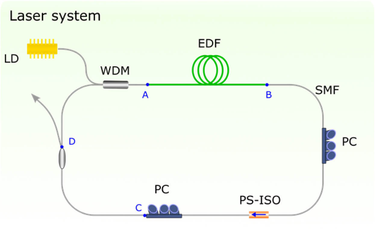
    Fig. 1. Schematic of the laser. EDF, erbium-doped fiber; LD, laser diode; WDM, wavelength-division multiplexer; PS-ISO, polarization-sensitive isolator; PC, polarization controller. Parameters for all cavity elements are given in the text.
    Transmittance of the laser cavity for three different cases. Case (i), the birefringence is switched off, and the wave plate angles are {2.372, 0.120, 0.035, 2.960} rad. Case (ii), the birefringence is switched on with LB=2 m, and the wave plate angles are {1.265, 0.5655, 1.508, 2.827} rad. Case (iii), the birefringence is switched on with LB=2 m, and the wave plate angles are {1.880, 0.1604, 0.7086, 2.787} rad. (a)–(c) Transmission spectra at low peak power (1 W, blue curve) and at high input peak power (450 W, green curve), which correspond to the left-side vertical axis; the red filled curve corresponding to the right-side vertical axis denotes the mode-locked soliton solution in each case. (d)–(f) Transmittance as a function of input peak power at three different wavelengths (1600 nm, 1613 nm, and 1625 nm). (a) and (d) correspond to case (i); (b) and (e) correspond to case (ii); (c) and (f) correspond to case (iii).
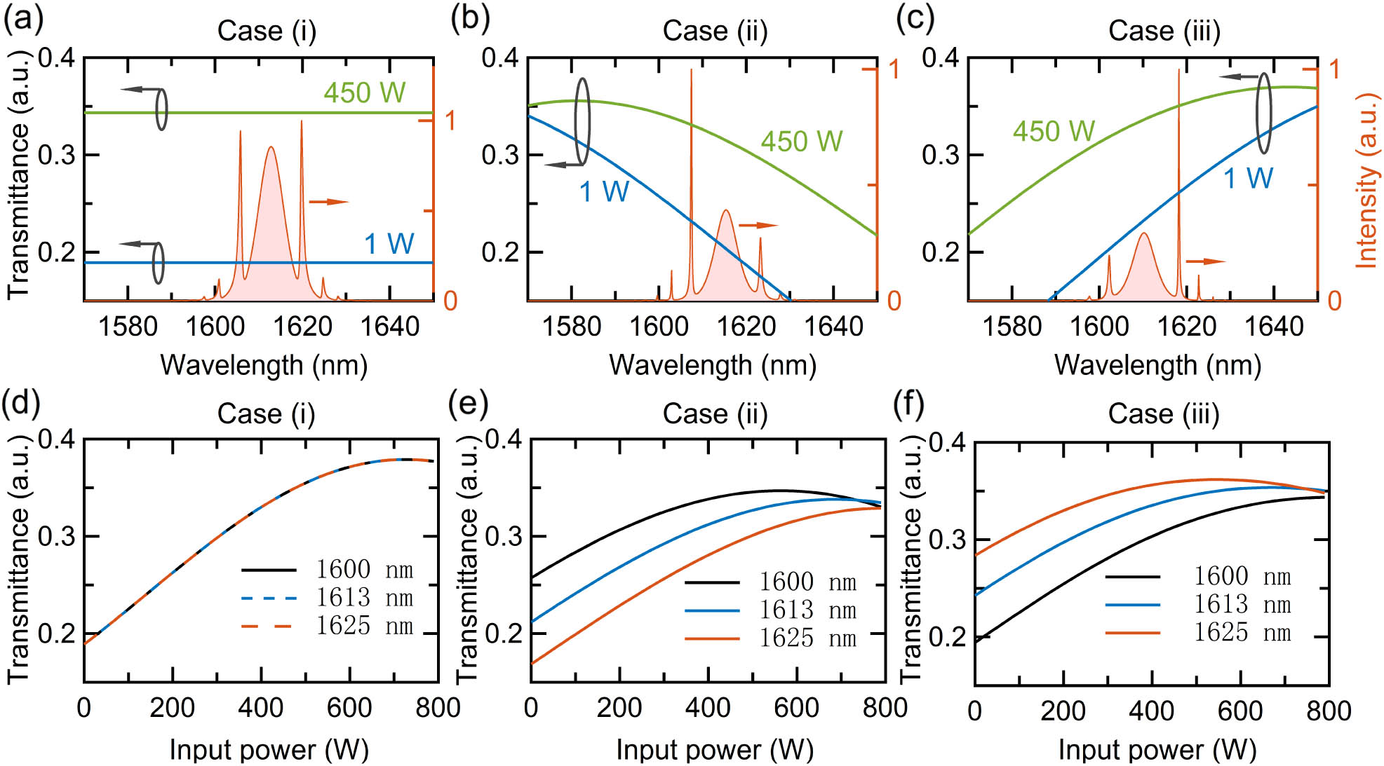
    Fig. 2. Transmittance of the laser cavity for three different cases. Case (i), the birefringence is switched off, and the wave plate angles are {2.372, 0.120, 0.035, 2.960} rad. Case (ii), the birefringence is switched on with LB=2  m, and the wave plate angles are {1.265, 0.5655, 1.508, 2.827} rad. Case (iii), the birefringence is switched on with LB=2  m, and the wave plate angles are {1.880, 0.1604, 0.7086, 2.787} rad. (a)–(c) Transmission spectra at low peak power (1 W, blue curve) and at high input peak power (450 W, green curve), which correspond to the left-side vertical axis; the red filled curve corresponding to the right-side vertical axis denotes the mode-locked soliton solution in each case. (d)–(f) Transmittance as a function of input peak power at three different wavelengths (1600 nm, 1613 nm, and 1625 nm). (a) and (d) correspond to case (i); (b) and (e) correspond to case (ii); (c) and (f) correspond to case (iii).
    Impact of gain profiles on resonant sideband generation. (a) Gain profiles obtained by superposing two Gaussian functions; the corresponding central wavelengths are 1579 nm and 1613 nm, and the bandwidths (FWHM) are 40.4 nm and 39.8 nm, respectively. The ratio of their weights c1/c4 is 0, 0.75, and 1.0, respectively, from the bottom to the top. (b) Spectrum of the mode-locked pulse for each gain profile when the birefringence is switched off, and the wave plate angles are the same as those in case (i) shown in Fig. 2. (c) Spectrum of the mode-locked pulse for each gain profile when the birefringence is switched on, and the wave plate angles are the same as those in case (ii) shown in Fig. 2.
    Fig. 3. Impact of gain profiles on resonant sideband generation. (a) Gain profiles obtained by superposing two Gaussian functions; the corresponding central wavelengths are 1579 nm and 1613 nm, and the bandwidths (FWHM) are 40.4 nm and 39.8 nm, respectively. The ratio of their weights c1/c4 is 0, 0.75, and 1.0, respectively, from the bottom to the top. (b) Spectrum of the mode-locked pulse for each gain profile when the birefringence is switched off, and the wave plate angles are the same as those in case (i) shown in Fig. 2. (c) Spectrum of the mode-locked pulse for each gain profile when the birefringence is switched on, and the wave plate angles are the same as those in case (ii) shown in Fig. 2.
    Evolution dynamics along the cavity. (a) Temporal and (b) spectral evolution of the pulse with multiple enhanced resonant sidebands. Labels A–D refer to the cavity positions in Fig. 1. The red curves on the vertical planes represent the temporal and spectral profiles of the pulse at the output coupler (point D). The dark dashed box in (a) highlights the main soliton, and the corresponding expanded view (on a linear scale) within a ∼3.3 ps time window is shown on the top of (a) as an inset.
    Fig. 4. Evolution dynamics along the cavity. (a) Temporal and (b) spectral evolution of the pulse with multiple enhanced resonant sidebands. Labels A–D refer to the cavity positions in Fig. 1. The red curves on the vertical planes represent the temporal and spectral profiles of the pulse at the output coupler (point D). The dark dashed box in (a) highlights the main soliton, and the corresponding expanded view (on a linear scale) within a 3.3ps time window is shown on the top of (a) as an inset.
    Characterization of the resonant sidebands. (a) Spectra of the soliton and resonant sidebands at the output coupler (point D) shown on a logarithmic scale. The inset corresponds to a linear scale visualization. (b) Wavelength of the resonant sideband (on the blue side of the soliton) as a function of the sideband order. The dark solid curve denotes the wavelengths of the sidebands [peak positions in (a)] obtained directly from the simulated spectrum. The filled red circles denote the sideband positions calculated with Eq. (4), and the filled blue circles denote the sideband positions calculated with Eq. (5). The inset represents the prediction error for the position of the resonant sideband with Eq. (4) (filled red triangles) and Eq. (5) (filled blue triangles). (c) Temporal profile of the pulse. The inset represents an expanded view of the main soliton, and the dashed cyan curve represents a hyperbolic secant soliton fit. (d) Expanded view of the temporal profile (filled dark curve) within a power range from 0 W to 5 W highlights the dispersive wave structures, which corresponds to that shown in the dashed box in (c); the red curve represents the superposition of S1, S2, and S3. (e) Temporal profiles of the first four orders of resonant sidebands filtered out; the inset corresponds to a logarithmic scale visualization. (f) Temporal evolution map (on a linear scale) of the superpositions of the first three orders of sidebands (S1 + S2 + S3).
    Fig. 5. Characterization of the resonant sidebands. (a) Spectra of the soliton and resonant sidebands at the output coupler (point D) shown on a logarithmic scale. The inset corresponds to a linear scale visualization. (b) Wavelength of the resonant sideband (on the blue side of the soliton) as a function of the sideband order. The dark solid curve denotes the wavelengths of the sidebands [peak positions in (a)] obtained directly from the simulated spectrum. The filled red circles denote the sideband positions calculated with Eq. (4), and the filled blue circles denote the sideband positions calculated with Eq. (5). The inset represents the prediction error for the position of the resonant sideband with Eq. (4) (filled red triangles) and Eq. (5) (filled blue triangles). (c) Temporal profile of the pulse. The inset represents an expanded view of the main soliton, and the dashed cyan curve represents a hyperbolic secant soliton fit. (d) Expanded view of the temporal profile (filled dark curve) within a power range from 0 W to 5 W highlights the dispersive wave structures, which corresponds to that shown in the dashed box in (c); the red curve represents the superposition of S1, S2, and S3. (e) Temporal profiles of the first four orders of resonant sidebands filtered out; the inset corresponds to a logarithmic scale visualization. (f) Temporal evolution map (on a linear scale) of the superpositions of the first three orders of sidebands (S1 + S2 + S3).
    Experimentally measured spectrum shown on a (a) logarithmic scale and (b) linear scale. The dashed vertical lines in (a) denote the sideband wavelengths predicted with Eq. (5), which takes the TOD effect into account. The inset in (b) shows a close-up view of the spectrum, which highlights the soliton. (c) Wavelength of the resonant sideband (on the blue side of the soliton) as a function of the sideband order. The dark curve denotes the wavelengths of the sidebands [peak positions in (a)] obtained directly from the measured spectrum. The filled red circles denote the sideband positions calculated with Eq. (4), and the filled blue circles denote the sideband positions calculated with Eq. (5). The inset represents the prediction error for the sideband positions with Eq. (4) (filled red triangles) and Eq. (5) (filled blue triangles). (d) Pulse train recorded with the oscilloscope.
    Fig. 6. Experimentally measured spectrum shown on a (a) logarithmic scale and (b) linear scale. The dashed vertical lines in (a) denote the sideband wavelengths predicted with Eq. (5), which takes the TOD effect into account. The inset in (b) shows a close-up view of the spectrum, which highlights the soliton. (c) Wavelength of the resonant sideband (on the blue side of the soliton) as a function of the sideband order. The dark curve denotes the wavelengths of the sidebands [peak positions in (a)] obtained directly from the measured spectrum. The filled red circles denote the sideband positions calculated with Eq. (4), and the filled blue circles denote the sideband positions calculated with Eq. (5). The inset represents the prediction error for the sideband positions with Eq. (4) (filled red triangles) and Eq. (5) (filled blue triangles). (d) Pulse train recorded with the oscilloscope.
    Typical spectra obtained by adjusting a quarter-wave plate angle. (a)–(c) Spectrum measured in the experiment at three different quarter-wave plate angles. (d)–(f) Wavelength of the resonant sideband (on the blue side of the soliton) as a function of the sideband order, which corresponds to the spectrum shown in (a)–(c), respectively. The solid dark curve denotes the sideband wavelengths obtained directly from the experimental spectrum. The filled red and blue circles denote the sideband positions calculated with Eq. (4) and Eq. (5), respectively. The inset in each subplot represents the prediction error with Eq. (4) (filled red triangles) and Eq. (5) (filled blue triangles). (g)–(i) Spectrum obtained from the numerical simulation with the wave plate angles of {1.243, 0.5655, 1.508, 2.827} rad, {1.268, 0.5655, 1.508, 2.827} rad, and {1.276, 0.5655, 1.508, 2.827} rad, respectively. (j)–(l) Wavelength of the resonant sideband (on the blue side of the soliton) as a function of the sideband order, which corresponds to the simulated spectrum shown in (g)–(i), respectively. The dark line denotes the sideband positions obtained directly from the numerical simulation. The filled red and blue circles denote the sideband positions calculated with Eq. (4) and Eq. (5), respectively. The inset in each plot represents the prediction error with Eq. (4) (filled red triangles) and Eq. (5) (filled blue triangles). The black curve on the top of (c) corresponding to the right vertical axis denotes the measured gain profile, and that on the top of (i) denotes the gain profile used in the simulation.
    Fig. 7. Typical spectra obtained by adjusting a quarter-wave plate angle. (a)–(c) Spectrum measured in the experiment at three different quarter-wave plate angles. (d)–(f) Wavelength of the resonant sideband (on the blue side of the soliton) as a function of the sideband order, which corresponds to the spectrum shown in (a)–(c), respectively. The solid dark curve denotes the sideband wavelengths obtained directly from the experimental spectrum. The filled red and blue circles denote the sideband positions calculated with Eq. (4) and Eq. (5), respectively. The inset in each subplot represents the prediction error with Eq. (4) (filled red triangles) and Eq. (5) (filled blue triangles). (g)–(i) Spectrum obtained from the numerical simulation with the wave plate angles of {1.243, 0.5655, 1.508, 2.827} rad, {1.268, 0.5655, 1.508, 2.827} rad, and {1.276, 0.5655, 1.508, 2.827} rad, respectively. (j)–(l) Wavelength of the resonant sideband (on the blue side of the soliton) as a function of the sideband order, which corresponds to the simulated spectrum shown in (g)–(i), respectively. The dark line denotes the sideband positions obtained directly from the numerical simulation. The filled red and blue circles denote the sideband positions calculated with Eq. (4) and Eq. (5), respectively. The inset in each plot represents the prediction error with Eq. (4) (filled red triangles) and Eq. (5) (filled blue triangles). The black curve on the top of (c) corresponding to the right vertical axis denotes the measured gain profile, and that on the top of (i) denotes the gain profile used in the simulation.
    Relative prediction error δ(ϵ,n) as a function of the sideband order n and ϵ obtained with (a) Eq. (A3) and (b) Eq. (A4). The red curve on each map denotes a 3 dB [δ(ϵ,n)=0.5] contour.
    Fig. 8. Relative prediction error δ(ϵ,n) as a function of the sideband order n and ϵ obtained with (a) Eq. (A3) and (b) Eq. (A4). The red curve on each map denotes a 3 dB [δ(ϵ,n)=0.5] contour.
    Sideband enhancement controlled by changing the pump power. Spectra measured at pump powers of (a) 200 mW, (b) 230 mW, (c) 280 mW, (d) 330 mW, (e) 380 mW, and (f) 400 mW. The spectral contrast between the most intense sideband and the soliton is highlighted in each subplot.
    Fig. 9. Sideband enhancement controlled by changing the pump power. Spectra measured at pump powers of (a) 200 mW, (b) 230 mW, (c) 280 mW, (d) 330 mW, (e) 380 mW, and (f) 400 mW. The spectral contrast between the most intense sideband and the soliton is highlighted in each subplot.
    Characterization of the stability of the mode-locked pulse with significantly enhanced sidebands measured at a pump power of 400 mW. (a) Spectra recorded every 15 min for 1 h. (b) Intensity difference (red balls, left vertical axis) and output power (bule balls, right vertical axis) recorded every 5 min during 1 h.
    Fig. 10. Characterization of the stability of the mode-locked pulse with significantly enhanced sidebands measured at a pump power of 400 mW. (a) Spectra recorded every 15 min for 1 h. (b) Intensity difference (red balls, left vertical axis) and output power (bule balls, right vertical axis) recorded every 5 min during 1 h.
    Tianqi Zhang, Fanchao Meng, Qi Yan, Chuanze Zhang, Zhixu Jia, Weiping Qin, Guanshi Qin, Huailiang Xu. Significant enhancement of multiple resonant sidebands in a soliton fiber laser[J]. Photonics Research, 2023, 11(11): 1847
    Download Citation