
Hong-Li Zeng, Erik Aurell. Inverse Ising techniques to infer underlying mechanisms from data[J]. Chinese Physics B, 2020, 29(8):
- Chinese Physics B
- Vol. 29, Issue 8, (2020)
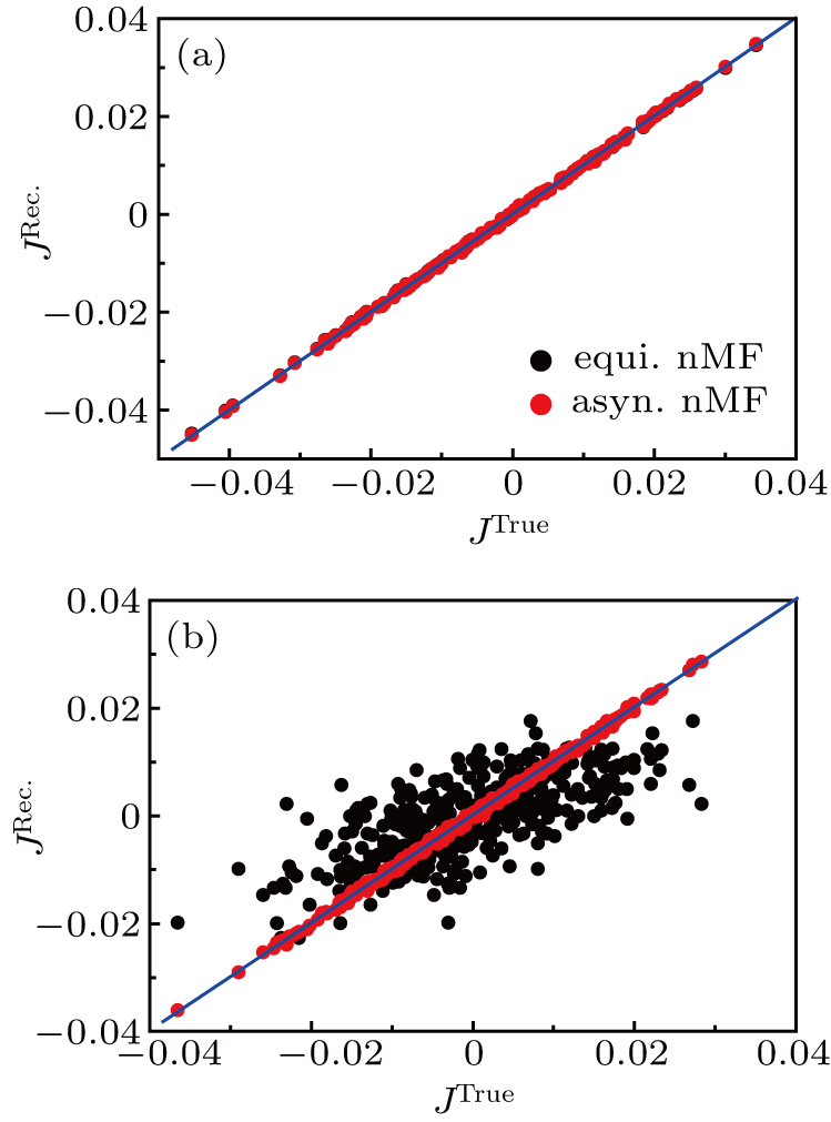
Fig. 1. The scatter plots for the true tested couplings versus the reconstructed ones. (a) Reconstruction for the symmetric SK model with k = 0; (b) inference for the asymmetric SK model with k = 1. Red dots, inferred couplings with asynchronous nMF approximation; black dots, inferred ones with equilibrium nMF approximation. The recovered asynchronous Jij ’s in (a) are symmetrized while no symmetrization for them in (b). The other parameters for both panels are g = 0.3, N = 20, θ = 0, L = 20 × 107.
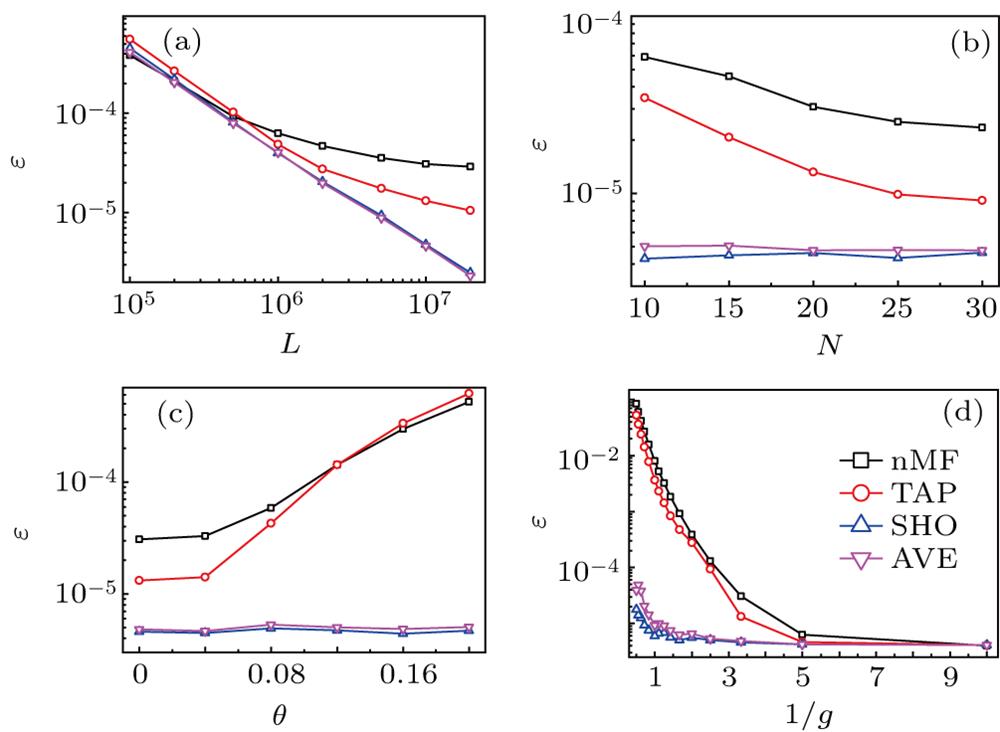
Fig. 2. Mean square error (ε ) versus (a) data length L , (b) system size N , (c) external field θ and (d) temperature 1/g . Black squares show nMF, red circles, TAP, blue up triangle SHO and pink down triangle AVE respectively. The parameters are g = 0.3, N = 20, θ = 0, L = 107 except when varied in a panel.
Fig. 3. Inferred asynchronous versus equilibrium couplings for retinal data. Red open dots show the self-couplings which by convention are equal to zero for the equilibrium model.
Fig. 4. Traded volume data for the stock of Fannie Mae (FNM), a mortgage company. Black line for time series of traded volumes Vi (t ), red for summed volumes during time interval Δt , blue for the threshold V i th = χ V i av × Δ t t = 50 s and χ = 1.
Fig. 5. Histograms of inferred couplings by equilibrium nMF and re-scaled asynchronous nMF. Black squares for re-scaled N (J asyn) to have the same standard deviation as N (J eq). Here χ = 0.5 and Δt = 200 s for both the methods.
Fig. 6. Histograms of the eigenvalues of the equal time connected correlation matrix. Parameters: χ = 0.5 and Δt = 100 s.
Fig. 7. Inferred financial networks, showing only the largest interaction strengths (proportional to the width of links and arrows). Colors are indicative, and chosen by a modularity-based community detection algorithm.[16 ] Parameters: χ = 0.5 and Δt = 100 s. (a) Equilibrium inference (the figure originates from Ref. [86 ]). (b) Asynchronous inference with τ = 20 s.
Fig. 8. (a) Temporal behavior of all allele frequencies defined as fi [1 ]. Data recorded every 5 generations. (b) An example of pairwise correlation changing with time. With finite population size, there exists strong fluctuations in the system. (c) Scatter plot for the reconstructed against the tested fitness with DCA-nMF (red dots) and DCA-PLM (blue dots) algorithm for Jij ’s. Parameters: the number of loci L = 25, the number of individuals N = 200, mutation rate μ = 0.01, recombination rate r = 0.1, crossover rate ρ = 0.5, standard deviation of epistatic fitness σ = 0.002.
Fig. 9. Phase diagram for epistatic fitness recovery with DCA-nMF Jij ’s from the average of singletime data. (a) Mutation rate μ versus recombination rate r . For large recombination while low mutation, KNS inference does not work. However, for small r , the KNS inference theory does not satisfied. (b) Epistatic fitness strength σ with r . For large recombination and very small fitness, KNS inference does not work.
Fig. 10. Scatter-plots of inferred epistatic fitness against the true fitness based on the averaged results from singletime: (a) with sad face: r = 0.1, where the KNS theory cannot be satisfied here, (b) with smiling face: r = 0.5, where inference works, (c) with not-that-sad face: r = 0.9, where the KNS theory works but with very heavy fluctuations. Here the DCA-nMF algorithm for Jij ’s is utilized.
Fig. 11. Corresponding scatter plots by alltime averages with Fig. 10 . The DCA-nMF algorithm for Jij ’s is also used here. The parameters for each sub-panel are the same as those in Fig. 10 .

Set citation alerts for the article
Please enter your email address
© Copyright 2018-2021 | Chinese Laser Press. All Rights Reserved 沪ICP备15018463号-20