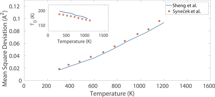
Fig. 1. Comparison of the atomic mean square deviation and Debye temperature, T_D, produced by interatomic potential developed by Sheng et al.³⁴ and the values obtained from x-ray diffraction measurements at equilibrium temperatures up to melting by Syneček et al.⁵⁴

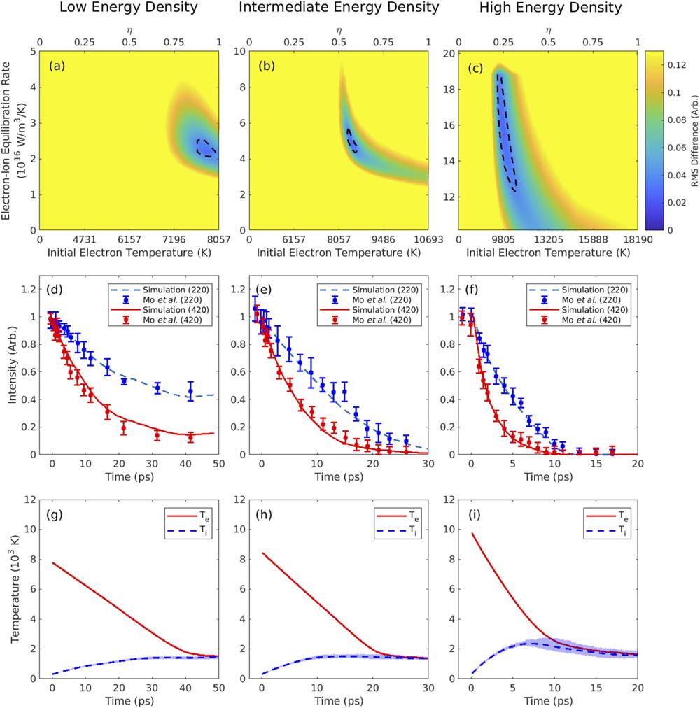
Fig. 2. Comparison between experimentally obtained Laue decay curves¹⁰ and those given by molecular dynamics simulations. (a)–(c) The rms difference between simulated and experimental decay curves for a range of initial electron temperatures and electron–ion equilibration rates. Here, the rms differences of the (220) and (420) curves have been added in quadrature. The area enclosed by the dashed line encompasses the region in which the simulation results lie within the experimental error bars. (d)–(f) Comparisons, for each energy density, of the experimental and simulated decays of the (220) and (420) Laue peaks for best-fit values of Te0 and g_ei obtained in (a)–(c). (g)–(i) The corresponding temporal evolutions of the electron and ion temperatures. Here, the area shaded in blue represents the variation in the ion temperature across the sample.

Fig. 3. (a) Evolution of best-fit values of η for several functional forms of the electron–ion equilibration rate.^{21–23,25,26,29} Here, Medvedev et al.* is used to denote the g_ei(T_e, T_i) prediction that is both electron- and ion-temperature-dependent. In our calculations of the average η for all theoretical models, we exclude the outlier results produced by the solely electron-temperature-dependent model calculated by Medvedev and Milov at a constant ion temperature of 300 K, and the Migdal et al. model. (b) Average value of g_ei for a given energy density up until melting. The value plotted has been calculated by taking the average over the g_ei value present out until 50, 25, and 10 ps in the low, intermediate, and high energy density cases, respectively.

Fig. 4. Comparison of simulated and measured spatially resolved diffraction pattern data for the low energy density case. (a)–(c) Spatially resolved data from the simulation for 100, 1000, and 3000 ps. (d) Angularly resolved diffraction data obtained from azimuthal integrals of the data shown in (a)–(c). (e)–(g) Spatially resolved data obtained by Mo et al.¹⁰ (h) Angularly resolved diffraction data obtained from azimuthal integrals of the data shown in (e)–(g).

Fig. 5. Same as Fig. 4, but for the intermediate energy density case and times of 20, 100, and 800 ps.

Fig. 6. Same as Fig.4, but for the high-energy density-case and times of −2, 7, and 17 ps.

Fig. 7. Visualization of gold melting in the low [(a)–(c)], intermediate [(d)–(f)], and high [(g)–(i)] energy density cases via the technique of polyhedral template matching⁷⁰ in OVITO visualization software.⁶⁹ For each energy density case, the time steps corresponding to the diffraction patterns shown in Figs. 4–6 are presented. The green color identifies the fcc lattice type, whereas the non-green colors identify liquid present in the sample. These results were produced using the smaller simulation geometry.

Fig. 8. Comparison between experimentally obtained Laue decay curves¹⁰ and those given by molecular dynamics simulations utilizing temperature-dependent electron–ion equilibration rates^{21–23,25,26,29} for the low (a), intermediate (b), and high (c) energy density cases. Here, “Medvedev et al.*” is used to denote a g_ei(T) prediction that is both electron- and ion-temperature-dependent.²³ For all three energy density cases, the rms difference between simulated and experimental decay curves for a range of initial electron temperatures is shown for each of the employed g_ei(T) models. In our analysis, the rms differences of the (220) and (420) curves have been added in quadrature.

Table 1. Experimentally measured properties of face-centered cubic (fcc) gold alongside those reproduced in molecular dynamics simulations using the interatomic potentials developed by Sheng et al. and the electron-temperature-dependent (ETD) potential of Norman et al. Here, the values shown for the Norman et al. potential are for the variant of the potential calculated for T_e ∼ 0.1 eV.