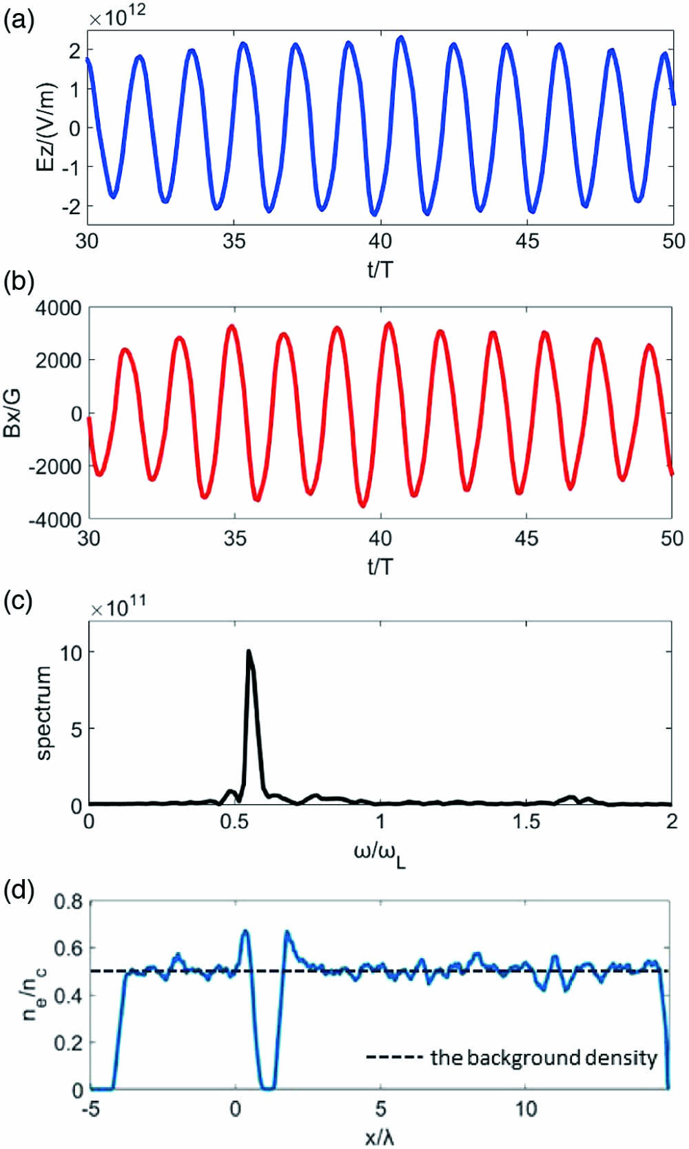
Fig. 1. Temporal evolution of (a) electric field and (b) magnetic field. The electric and magnetic fields are oscillated periodically, and the magnetic field lags quarter of an oscillation period behind the electric field. Panel (c) shows the Fourier transformation of the electric field from 0 T to 60 T, i.e., the spectrum of the soliton. There is a monoenergetic peak in frequency domain referring to the soliton frequency. Panel (d) is the lineout of longitudinal density of the electrons. The vacuum–plasma interface is at −4λ, and the density valley around 1λ is where the soliton position is. The localized density on either side of the valley is slightly higher than the background density.

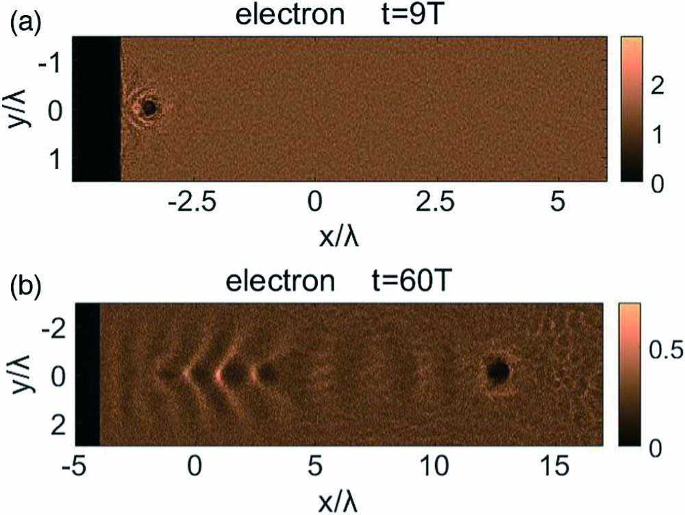
Fig. 2. Distributions of electrons in the cases of (a) density close to upper limit and (b) lower limit of soliton generation for a = 1. The units of density, time, and length are critical plasma density, laser period, and wavelength, respectively. The soliton in panel (a) stays stationary near the interface, while the soliton in panel (b) stays at some distance away from the interface. The periodic density hump between vacuum–plasma interface and the soliton in panel (b) is the trail of the laser wakefield. It is obvious that the size of the two solitons is different.

Fig. 3. Relationship between plasma density and the distance from the position of the solitons to the vacuum–plasma interface is drawn. For a fixed normalized value a = 1, the distance from the interface of the solitons decreases with an increase in the number density of electrons. The red solid curve is more consistent with the simulation results than the gray dotted curve.

Fig. 4. Panel (a) shows the upper and lower density limits of the existence of solitons at the wavelength of 3 microns. Panel (b) is the existence of solitons at different wavelengths. The abscissa is the intensity of the incident laser, and the ordinate is the density of the plasma. Brown, blue, and black represent the existence criteria of EM solitons when the wavelength of the incident laser is 30 mm, 300 µm, and 3 µm, respectively.

Fig. 5. Composition of the proposed experiment to induce expectant ball lightning EM solitons with high-field THz.