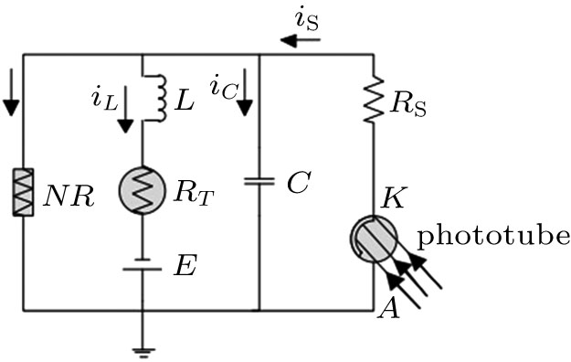
Fig. 1. Schematic diagram for the neural circuit, which is dependent on the illumination and temperature. NR is a nonlinear resistor, C is the capacitor, L represents an induction coil, R_T denote a thermistor, R and R_S are linear resistors, and E is a constant voltage source. K denotes the cathode and A represents the anode in the phototube. The relation between the resistance of thermistor and temperature T is estimated with R_T = R_∞ exp(B/T), and the material parameter B is determined by the activation energy q and the Boltzmann’s constant K′ with the dependence as B = q/K′.

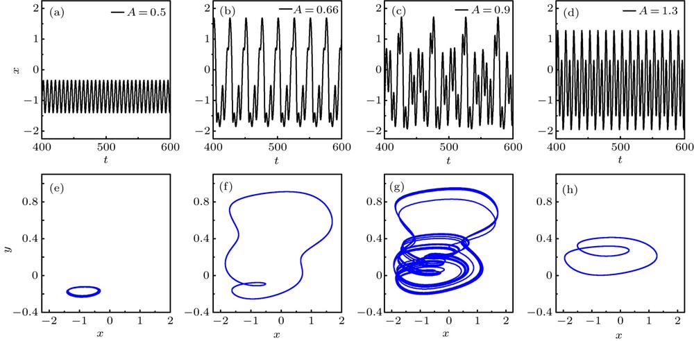
Fig. 2. Sampled time series for variable x and formation of attractors: (a), (e) A = 0.5; (b), (f) A = 0.66; (c), (g) A = 0.9; (d), (h) A = 1.3, and the parameters are fixed at T′ = 5, u₀ = 0.2, ω = 1.004, b₀ = 0.8, a = 0.7, c = 0.1, ξ = 0.175. b₀ is the maximal resistance of the thermistor.

Fig. 3. Sampled time series for variable x and formation of attractors: (a), (e) A = 0.76; (b), (f) A = 0.83; (c), (g) A = 0.99; (d), (h) A = 1.36, and the parameters are fixed at T′ = 1, u₀ = 0.2, ω = 1.004, b₀ = 0.8, a = 0.7, c = 0.1, ξ = 0.175. b₀ is the maximal resistance of the thermistor.

Fig. 4. Bifurcation diagram is calculated by detecting interspike intervals (ISIs) from the sampled time series for the variable x when the amplitude of voltage source is changed: (a) T′ = 0.5; (b) T′ = 1; (c) T′ = 5; (d) T′ = 20, and the parameters are fixed at u₀ = 0.2, ω = 1.004, b₀ = 0.8, a = 0.7, c = 0.1, ξ = 0.175.

Fig. 5. (a)–(c) Sampled time series for variable x, (d)–(f) formation of attractors, and (g) bifurcation diagram vs. angular frequency. For (a), (d) ω = 0.005; (b), (e) ω = 0.01; (c), (f) ω = 0.05, and the parameters are fixed at T′ = 10, A = 1, u₀ = 0.2, b₀ = 0.8, a = 0.7, c = 0.1, ξ = 0.175.

Fig. 6. Bifurcation diagram is calculated by detecting ISIs from the sampled time series for the variable x when the frequency of voltage source is changed: (a) T′ = 0.5; (b) T′ = 1; (c) T′ = 5; (d) T′ = 10, and the parameters are fixed at u₀ = 0.2, A = 1, b₀ = 0.8, a = 0.7, c = 0.1, ξ = 0.175.

Fig. 7. Bifurcation diagram is calculated by detecting ISIs from the sampled time series for the variable x when the amplitude of thermistor is changed: (a) T′ = 0.5; (b) T′ = 1; (c) T′ = 5; (d) T′ = 10, and the parameters are fixed at u₀ = 0.2, A = 1, ω = 1.004, b₀ = 0.8, a = 0.7, c = 0.1, ξ = 0.175.

Fig. 8. Bifurcation diagram is calculated by detecting ISIs from the sampled time series for the variable x when the temperature for thermistor is changed: (a) b₀ = 0.6; (b) b₀ = 0.7; (c) b₀ = 0.8; (d) b₀ = 0.9, and the parameters are fixed at u₀ = 0.2, A = 1, ω = 1.004, a = 0.7, c = 0.1, ξ = 0.175.

Fig. 9. Correlation between temperature, resistance of thermistor, firing patterns and Hamilton energy are calculated by changing the temperature of the thermistor. For (a1)–(a4) b₀ = 0.1; (b1)–(b4) b₀ = 0.4; (c1)–(c4) b₀ = 0.6, and the parameters are fixed at u₀ = 0.2, A = 1, ω = 1.004, a = 0.7, c = 0.1, ξ = 0.175.

Fig. 10. Firing pattern and photocurrent are calculated as functions of time by applying different temperatures for the thermistor. For (a) T′ = 10; (b) T′ = 30, and the parameters are fixed at I₀ = 0.05, b₀ = 0.3, a = 0.7, c = 0.1, ξ = 0.175, v_a = 1 (black line), v_a = 0.1 (red line). The photocurrent is released from t = 200 time units.

Fig. 11. Mean duration of spiking is calculated by changing the parameters (I₀, T′) with b₀ = 0.3, T′ = 10 (red line-square), T′ = 20 (orange line-circle), T′ = 30 (violet line-up triangle). For (a) I₀ = 0.1; (b) v_a = 0.1.

Fig. 12. Bifurcation diagram is calculated by detecting ISIs from the sampled time series for the variable x when the amplitude for photocurrent is changed. For (a) v_a = 1.0; (b) v_a = 0.1, and the parameters are fixed at b₀ = 0.3, T′ = 10 (black dots), T′ = 30 (red dots), a = 0.7, c = 0.1, ξ = 0.175.

Fig. 13. Bifurcation diagram is calculated by detecting ISIs from the sampled time series for the variable x when the inverse threshold for photocurrent is changed. The parameters are fixed at b₀ = 0.3, I₀ = 0.2, T′ = 10 (black dots), T′ = 20 (red dots), T′ = 30 (blue dots), a = 0.7, c = 0.1, ξ = 0.175.

Fig. 14. Correlation between temperature, resistance of thermistor, firing patterns and Hamilton energy are calculated by changing the temperature for the thermistor. For (a1)–(a4) b₀ = 0.1; (b1)–(b4) b₀ = 0.3; (c1)–(c4) b₀ = 0.5, and the parameters are fixed at I₀ = 0.05, v_a = 1.0, a = 0.7, c = 0.1, ξ = 0.175.

Fig. 15. (b) Sampled time series for the variable x and (c) attractor are calculated when the temperature for the thermistor is adjusted as (a) T′ = 10.2 + 10 cos 0.1001τ. The parameters are selected as a = 0.7, c = 0.1, ξ = 0.175, I_S = 0.0, b₀ = 0.01.

Fig. 16. (c) Sampled time series for the variable x and (b) resistance of thermistor are calculated when the temperature for thermistor is adjusted as (a) T′ = 10.2 + 10 cos 0.01τ. The parameters are selected as a = 0.7, c = 0.1, ξ = 0.175, I_S = 10 arctan(25x – 10), b₀ = 0.01.

Fig. 17. Coefficient variability of ISI series is calculated by changing the noise intensity when the phototube is used as voltage source. The parameters are fixed at a = 0.7, c = 0.1, ξ = 0.175, u₀ = 0.2, A = 0.76, ω = 1.004, b₀ = 0.8, T’ = 1. During getting the average ISI, the threshold for peaks is selected as 0.3.

Fig. 18. Coefficient variability of ISI series is calculated by changing the noise intensity when the phototube is used as current source. The parameters are fixed at a = 0.7, c = 0.1, ξ = 0.175, I₀ = 0.19, v_a = 1, b₀ = 0.3, T’ = 10. During getting the average ISI, the threshold for peaks is selected as 0.3.