Abstract
Phase is a fundamental resource for optical imaging but cannot be directly observed with intensity measurements. The existing methods to quantify a phase distribution rely on complex devices and structures and lead to difficulties of optical alignment and adjustment. We experimentally demonstrate a phase mining method based on the so-called adjustable spatial differentiation, by analyzing the polarization of light reflection from a single planar dielectric interface. Introducing an adjustable bias, we create a virtual light source to render the measured images with a shadow-cast effect. From the virtual shadowed images, we can further recover the phase distribution of a transparent object with the accuracy of 0.05λ RMS. Without any dependence on wavelength or material dispersion, this method directly stems from the intrinsic properties of light and can be generally extended to a broad frequency range.1 Introduction
Phase distribution plays the key role in biological and x-ray imaging, where the information on objects or structures is mainly stored in phase rather than intensity variations. Phase distribution cannot be directly retrieved from conversional intensity measurements. Zernike invented the phase contrast microscopy1 to render the transparent objects but without the ability to quantify the phase distribution. Later, in order to enhance the image contrast, Nomarski prisms were created for differential interference contrast (DIC) imaging,2 which offers the phase gradient information. Based on Fourier optics, a differentiation filter3–5 or spiral phase filter6–9 in 4f system can visualize the phase of optical wavefront. Further, various quantitative phase measurement technologies10 based on the beam interference11–16 and propagation17–20 were developed for mapping the optical thickness of specimens. However, these methods usually rely on complex modulation devices in the spatial or spatial frequency domains, resulting in the difficulties of optical alignment and adjustment.
In recent years, optical analog computing of spatial differentiation has attracted great attention, which enables an entire image process on a single shot.21–31 Various optical analog computing devices were designed for edge detection.32–44 In particular, Silva et al. theoretically proposed realization of optical mathematical operations with metamaterials, as well as the Green’s function slabs.21 Later, a subwavelength-scale plasmonic differentiator of a 50-nm-thick silver layer was experimentally demonstrated and applied for real-time edge detection.32 Most recently, spatial differentiation methods were developed based on the geometric phases, including the Rytov–Vladimirskii–Berry phase40 and the Pancharatnam–Berry phase.41,45 So far, the current application of optical spatial differentiation is only limited to edge detection. As the fundamental difficulty to determine the phase of electric fields by measuring their intensities, one cannot determine the sign of the differentiation signal and hence recover the phase distributions.
In this article, we propose an adjustable spatial differentiation to characterize and quantitatively recover the phase distribution, just by simply analyzing the polarization of light reflection from a single planar dielectric interface. By investigating the field transformation between two linear cross polarizations, we experimentally demonstrate that the light reflection enables an optical analog computing of spatial differentiation with adjustable direction. We show that this effect is related to the angular Goos–Hänchen (GH) shift46–48 and the Imbert–Fedorov (IF) shift.49,50 Furthermore, by tuning a uniform constant background as the bias, we create a virtual light source to render the measured images with a shadow-cast effect and further quantify the phase distribution of a coherent field within accuracy. Without complex modulation devices,3–9,11–14 our method offers great simplicity and flexibility, which can circumvent the fabrication of complex structures and also the difficulties of optical alignment and adjustment. Importantly, since the proposed method is irrelevant to resonance or material dispersion, it works at general wavelengths with large temporal bandwidths, which is very suitable for high-throughput real-time image processing.
Sign up for Advanced Photonics TOC. Get the latest issue of Advanced Photonics delivered right to you!Sign up now
2 Adjustable Spatial Differentiation
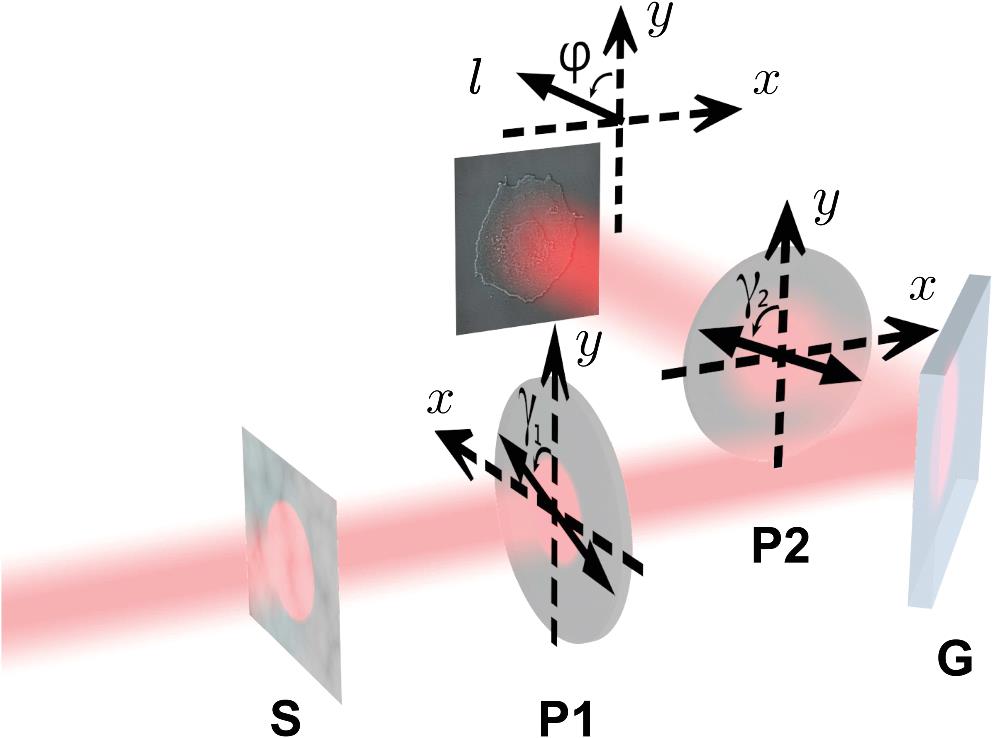
Schematically shown as Fig. 1, the proposed phase mining scheme only includes a dielectric interface as a planar reflector and two polarizers P1 and P2, where the incident light is assuming a phase distribution . Next we show that such a light reflection process can transform the original uniform intensity image with invisible phase structure into a structured contrast image, by optical computing of spatial differentiation to the incident electric field. Moreover, the direction of the spatial differentiation can be further adjusted with different combinations of the polarizer orientation angles.

Figure 1.Schematic of the phase-mining method based on polarization analysis of light reflection on a dielectric interface, e.g., an air–glass interface. A phase object S is uniformly illuminated and then the light is polarized by a polarizer P1 and reflected on the surface of a glass slab G. By analyzing the polarization of the reflected light with a polarizer P2, the differential contrast image of S appears at the imaging plane of the system and can exhibit a shadow-cast effect. The polarizers P1 and P2 are orientated at the angles and . The direction of the spatial differentiation is along and indicated with an angle .
To specifically depict the transformation, we decompose the incident (output) beam into a series of plane waves as according to spatial Fourier transform. Then, the spatial transformation between the measured field and the original one is determined by a spatial spectral transfer function . We denote the orientation angles of the polarizers P1 and P2 as and , respectively. The spatial spectral transfer function can be written as (see Sec. 1 in the Supplemental Material) where and are the Fresnel reflection coefficients of the - and -polarized plane waves, respectively. In Eq. (1), the third term is induced by the opposite -directional displacements for left- and right-handed circularly polarized beams, which is known as the IF shift.40,51 By considering the GH effect, we expand the () around the incident angle as , where is the Fresnel reflection coefficient for the central plane wave, and is the wavevector number in vacuum. We note that here such a spatial dispersion during partial reflection on the dielectric interface purely leads to an angular GH shift.46–48
For a partial reflection process on a dielectric interface, we can control the orientation angle of the polarizers P1 and P2 to satisfy the cross-polarization condition In such a condition, the P2 polarizer is oriented orthogonally to the polarization of the reflected central plane wave, which is first polarized by P1 and then reflected by the dielectric interface with an incident angle . Under the cross-polarization condition, the spatial spectral transfer function becomes where and are two coefficients as and . Equation (3) shows that the spatial spectral transfer function is linearly dependent on the spatial frequencies and , which corresponds to the computation of a directional differentiation in the spatial domain: . We note that the directional spatial differentiation occurs in every oblique partial reflection case on a dielectric interface, but hardly in total internal reflection or metallic reflection cases where the complex and prevent the satisfaction of Eq. (2). Besides, since and in Eq. (3) are also complex, the directional differentiation no longer exists unless is purely real.
Considering the original field , the output field is which offers a differential contrast image of the phase object along direction defined as . Besides, the coefficient in Eq. (4) varies with different directions (see Sec. 3 in the Supplemental Material), which is a quantitatively important coefficient when utilizing spatial differentiation along different directions in the meantime.
We note that the direction , described by an angle as shown in Fig. 1, is continuously adjustable with different values of and . Under a certain incident angle, the direction angle varies with different pairs of and that satisfy the cross-polarization condition. We note that only when the incident angle is smaller than Brewster angle, can cover a complete range from 0 deg to 180 deg. However, when the incident angle is larger than Brewster angle, both and become negative, and hence the coefficients and are always negative and in a limited range so that the corresponding values of are also limited.
3 Bias Introduction and Phase Mining
We note that even though the edges of phase objects can be detected through the directional differentiation along direction , the sign of the differentiation cannot be distinguished since the measured intensity is proportional to . It means the edges cannot be determined as the ridges or the troughs in the phase structure. In order to determine the sign of the differentiation, we add a uniform constant background as a bias into the proposed spatial differentiation and generate contrast images with shadow-cast effect. We show that the bias can be easily introduced and adjusted in the proposed phase quantifying scheme, in comparison to the other methods, such as traditional DIC microscopy2,52 or spiral phase contrast microscopy.
The uniform constant background is introduced by breaking the spatial differentiation requirement of Eq. (2), that is, by rotating the polarizers for a small angle deviating from the cross-polarization condition. In this case, Eq. (2) is changed to where is a constant and continuously adjustable with and .
Following the same way as Eqs. (3) and (4), after introducing the uniform constant background, the measured reflected image is changed to (see the details in Sec. 4 of the Supplemental Material) and becomes shadow-cast. The sign of can be determined from the change of intensity. For example, with a positive bias , the intensity appears brighter (darker) in the areas with positive (negative) directional derivative . The biased image exhibits a shadow-cast effect, which appears as illuminated by a virtual light source, as schematically shown in Fig. 4(c).
Finally, we can recover the phase distribution with both the determined sign and the absolute value of . We implement the retrieval of phase distribution through a two-dimensional (2-D) Fourier method.53 It first requires two orthogonal directional derivatives, for example, the partial derivatives and . Then, we combine them as a complex distribution . In spatial frequency domain, its 2-D Fourier transform is . Therefore, the phase distribution can be recovered as
4 Experimental Demonstration
To demonstrate the proposed phase quantifying, we use a green laser source with wavelength and a BK7 glass slab with refractive index 1.5195 for reflection. According to Eqs. (1)–(3), we first simulate the adjustable range of under every different incident angle and the chosen orientation angle of P1. As shown in Fig. 2(a), the direction angle can be fully adjustable from 0 deg to 180 deg only when the incident angle is smaller than the Brewster angle (black dashed line).
Figure 2.Adjustability demonstration of the direction angle . As an example, here the source is a green laser with wavelength in vacuum and a BK7 glass slab with refractive index 1.5195 is used for reflection. (a) Adjustable range of direction angle under a certain incident angle with different pairs of and satisfying the cross-polarization condition. The white and black dashed lines correspond to and the Brewster angle, respectively. The points c to f on the white dashed line correspond to , 90 deg, 135 deg, and 180 deg, respectively. On the white dashed line in (a), . (b) Specific values of and for a certain direction angle . The points c to f are the same as those in (a), corresponding to , 90 deg, 135 deg, and 180 deg, respectively.
In order to show a complete adjustable range from 0 deg to 180 deg, we select an incident angle [the white dashed line in Fig. 2(a)]. We next experimentally demonstrate spatial differentiation for the direction angles , 90 deg, 135 deg, and 180 deg, by choosing the appropriate orientation angles and (see specific values in Sec. 5 of the Supplemental Material). By the requirement of Eq. (2), Fig. 2(b) gives the specific values of and . The points c to f in Figs. 2(a) and 2(b) correspond to the cases with these four direction angles , respectively.
As shown in Figs. 3(a)–3(d), the experiment demonstrates the edge-enhanced differential contrast imaging for a disc phase distribution [shown as the inset in Fig. 3(a)], with and for the differentiation direction , 90 deg, 135 deg, and 180 deg. Figures 3(a)–3(d) clearly exhibit the edges of the disc pattern as a circle, except the parts that are parallel to the differentiation direction. These results indeed show the adjustability of the direction of spatial differentiation.
Figure 3.Measurement of spatial differentiation results and corresponding spatial spectral transfer functions along different directions. (a)–(d) Measured spatial differentiation results of the phase distribution [the inset in (a)] along different directions with , 90 deg, 135 deg, and 180 deg, corresponding to points c to f in Fig. 2(a), respectively. The inset in (a) is a disc test pattern with different phases for the gray and the white areas. (e)–(h) Experimental results of spatial spectral transfer functions, corresponding to (a)–(d). (i)–(l) Corresponding theoretical results calculated based on Eq. (3).
For an accurate evaluation of the spatial differentiation direction, we experimentally measure the spatial spectral transfer functions as shown in Figs. 3(e)–3(h) (see the detailed procedures in Sec. 2 of the Supplemental Material). As Eq. (3) expects, Figs. 3(e)–3(h) indeed exhibit linear dependences on both and . For each case, the measured direction angles are 45.11 deg, 90.01 deg, 134.91 deg, and 180.00 deg, respectively, which are determined by fitting the gradient directions of the experimentally measured spatial spectral transfer functions (see Sec. 3 of the Supplemental Material). The measured results are shown as the arrows in Figs. 3(e)–3(h), respectively. For comparison, the theoretical spatial spectral transfer functions are calculated from Eq. (3) and shown in Figs. 3(i)–3(l), respectively; these functions agree well with the experimental ones. With the figure of merit (FOM) defined in Ref. 54, even though the bandwidth and gain of spatial differentiation vary with the differentiation direction, the FOM of the vertical one is 0.679. We note that specifically when or 90 deg, the spatial differentiation is only from the IF shift and exhibits vertically as or 180 deg. It becomes totally horizontal for , where the spatial differentiation is purely induced by the angular GH shift since the coefficient of the vertical spatial differentiation is .
Next, we experimentally demonstrate the biased imaging for a transparent phase object, by introducing a uniform constant background as the bias. According to Eq. (5), we first simulate the bias value as shown in Fig. 4(a), where the black dashed line corresponds to , i.e., the cross-polarization condition is satisfied. In order to demonstrate the biased effect, we generate the phase distribution of the incident light with a reflective phase-only spatial light modulator (SLM). An epithelial cell’s image55 in Fig. 4(b) is loaded into SLM, with a prior quantitative phase distribution. We introduce the bias by only controlling the value of deviating from the black dashed line to red triangle points in Fig. 4(a). The specific deviation angles of are 9 deg, 5 deg, 2 deg, and 1 deg, corresponding to bias values , 0.0151, 0.0100, and 0.0054, respectively (see Sec. 5 of the Supplemental Material). As shown in Figs. 4(d)–4(g), the results show the biased contrast images, which seem to result from a virtual light source obliquely illuminating the object along different directions [schematically shown in Fig. 4(c)]. These shadow-cast images result from the positive biases that render the ridges and the troughs in phase distribution as the bright edges and the shadowed ones, respectively.
Figure 4.Experimental demonstration of bias introduction and shadow-cast effect in differential contrast imaging of phase objects. (a) Theoretically calculated bias values under different and . The black dashed curve corresponds to the cross-polarization condition, where the bias value . (b) Phase distribution on the SLM, converted from an epithelial cell’s image. (c) Schematic of a virtual light source obliquely illuminating an object (green). The shadow-cast effects with virtual illumination from the points d to g schematically correspond to those in the biased images (d)–(g). (d)–(g) Measured biased differential contrast images with positive bias values corresponding to the triangle points d to g in (a), with bias values , 0.0151, 0.0100, and 0.0054, respectively. The white arrows indicate the orientations of the shadow cast in measured images. The white bars correspond to the length of .
With a positive and very small bias as a perturbation, we can determine the sign of the spatial differentiation . The absolute value of can be obtained from the nonbias case, and therefore we experimentally acquire the first-order directional derivatives of (see the details in Sec. 6 in the Supplemental Material). Figures 5(a) and 5(b) show two directional derivatives of the incident phase distribution shown as Fig. 4(b) along - and -directions, respectively. For comparison, the ideal spatial differentiations along - and -directions are calculated as Figs. 5(c) and 5(d), respectively. These experimental results clearly coincide well with the calculated ones, indicating great accuracy of the performance. Finally, we recover the phase from the obtained directional derivatives through the 2-D Fourier algorithm. Figure 5(e) shows the result of the recovered phase distribution, which coincides with the original incident one [Fig. 5(f)]. The root mean square (RMS) between the recovered result and the original distribution is calculated as , which can be further reduced with an optimized image system. In this way, we not only enhance the contrast to make transparent objects visible but also successfully recover its original phase distribution.
Figure 5.Directional derivatives of phase distribution in Fig. 4(b) and the corresponding recovered phase. Experimental results of (a) vertical and (b) horizontal partial derivatives of phase distribution in Fig. 4(b). Ideal (c) vertical and (d) horizontal partial derivatives. (e) Recovered phase distribution from (a) and (b) using the 2-D Fourier algorithm. (f) Original phase distribution on the SLM [the same as Fig. 4(b)].
5 Conclusion
We experimentally demonstrated a phase mining method only by analyzing the polarization of light reflection from a single planar dielectric interface. The direction of the spatial differentiation is continuously adjustable assuring differential contrast enhancement along different directions. Importantly, the method easily introduces a bias and generates shadow-cast differential contrast images. Based on this bias scheme, we determine the sign of the spatial differentiation of the phase distribution and finally recover the original phase information for a uniform-intensity image.
We note that the present method is also suitable for birefringent specimens with advantages over conventional DIC, because the illumination happens before polarization analysis in light reflection on a dielectric interface. This planar-interface scheme is much simpler and almost costless in comparison to the methods with complex Nomarski prisms or SLMs. Without the requirement of rotating the objects, the adjustability of differentiation direction works in situ and hence circumvents the difficulties and errors by using image registration. This method also works under a partially coherent illumination. For example, here a partially coherent beam is used for illumination of the phase object, in order to eliminate speckles and enhance the image quality. Our experimental results confirm that the proposed method is independent of material and wavelength, and therefore, by x-ray or electron polarization analysis,56,57 it opens a new avenue to quantify the phase in x-ray or electron microscopy imaging.
References
[1] F. Zernike. How I discovered phase contrast. Science, 121, 345-349(1955).
[2] R. Allen, G. David, G. Nomarski. The Zeiss-Nomarski differential interference equipment for transmitted-light microscopy. Z. Wiss. Mikrosk. Mikrosk. Tech., 69, 193-221(1969).
[3] H. Furuhashi, K. Matsuda, C. P. Grover. Visualization of phase objects by use of a differentiation filter. Appl. Opt., 42, 218-226(2003).
[4] D. Schmidt et al. Optical wavefront differentiation: wavefront sensing for solar adaptive optics based on a LCD. Proc. SPIE, 6584, 658408(2007).
[5] H. Furuhashi et al. Phase measurement of optical wavefront by an SLM differentiation filter(2009).
[6] J. A. Davis et al. Image processing with the radial Hilbert transform: theory and experiments. Opt. Lett., 25, 99-101(2000).
[7] S. Fürhapter et al. Spiral phase contrast imaging in microscopy. Opt. Express, 13, 689-694(2005).
[8] A. Jesacher et al. Shadow effects in spiral phase contrast microscopy. Phys. Rev. Lett., 94, 233902(2005).
[9] X. Qiu et al. Spiral phase contrast imaging in nonlinear optics: seeing phase objects using invisible illumination. Optica, 5, 208-212(2018).
[10] Y. Park, C. Depeursinge, G. Popescu. Quantitative phase imaging in biomedicine. Nat. Photonics, 12, 578-589(2018).
[11] T. Ikeda et al. Hilbert phase microscopy for investigating fast dynamics in transparent systems. Opt. Lett., 30, 1165-1167(2005).
[12] G. Popescu et al. Diffraction phase microscopy for quantifying cell structure and dynamics. Opt. Lett., 31, 775-777(2006).
[13] T. J. McIntyre et al. Differential interference contrast imaging using a spatial light modulator. Opt. Lett., 34, 2988-2990(2009).
[14] C. Zheng et al. Digital micromirror device-based common-path quantitative phase imaging. Opt. Lett., 42, 1448-1451(2017).
[15] P. Ferraro et al. Quantitative phase-contrast microscopy by a lateral shear approach to digital holographic image reconstruction. Opt. Lett., 31, 1405-1407(2006).
[16] C. J. Mann et al. High-resolution quantitative phase-contrast microscopy by digital holography. Opt. Express, 13, 8693-8698(2005).
[17] A. Barty et al. Quantitative optical phase microscopy. Opt. Lett., 23, 817-819(1998).
[18] H. M. L. Faulkner, J. Rodenburg. Movable aperture lensless transmission microscopy: a novel phase retrieval algorithm. Phys. Rev. Lett., 93, 023903(2004).
[19] S. S. Kou et al. Transport-of-intensity approach to differential interference contrast (TI-DIC) microscopy for quantitative phase imaging. Opt. Lett., 35, 447-449(2010).
[20] C. Zuo et al. Noninterferometric single-shot quantitative phase microscopy. Opt. Lett., 38, 3538-3541(2013).
[21] A. Silva et al. Performing mathematical operations with metamaterials. Science, 343, 160-163(2014).
[22] A. Pors, M. G. Nielsen, S. I. Bozhevolnyi. Analog computing using reflective plasmonic metasurfaces. Nano Lett., 15, 791-797(2014).
[23] L. L. Doskolovich et al. Spatial differentiation of optical beams using phase-shifted Bragg grating. Opt. Lett., 39, 1278-1281(2014).
[24] Z. Ruan. Spatial mode control of surface plasmon polariton excitation with gain medium: from spatial differentiator to integrator. Opt. Lett., 40, 601-604(2015).
[25] S. Abdollahramezani et al. Analog computing using graphene-based metalines. Opt. Lett., 40, 5239-5242(2015).
[26] A. Chizari et al. Analog optical computing based on a dielectric meta-reflect array. Opt. Lett., 41, 3451-3454(2016).
[27] A. Youssefi et al. Analog computing by Brewster effect. Opt. Lett., 41, 3467-3470(2016).
[28] Y. Hwang, T. J. Davis. Optical metasurfaces for subwavelength difference operations. Appl. Phys. Lett., 109, 181101(2016).
[29] Y. Fang, Y. Lou, Z. Ruan. On-grating graphene surface plasmons enabling spatial differentiation in the terahertz region. Opt. Lett., 42, 3840-3843(2017).
[30] W. Wu et al. Multilayered analog optical differentiating device: performance analysis on structural parameters. Opt. Lett., 42, 5270-5273(2017).
[31] Y. Hwang et al. Plasmonic circuit for second-order spatial differentiation at the subwavelength scale. Opt. Express, 26, 7368-7375(2018).
[32] T. Zhu et al. Plasmonic computing of spatial differentiation. Nat. Commun., 8, 15391(2017).
[33] J. Zhang, Q. Ying, Z. Ruan. Time response of plasmonic spatial differentiators. Opt. Lett., 44, 4511-4514(2018).
[34] Y. Fang, Z. Ruan. Optical spatial differentiator for a synthetic three-dimensional optical field. Opt. Lett., 43, 5893-5896(2018).
[35] A. Saba et al. Two dimensional edge detection by guided mode resonant metasurface. IEEE Photonics Technol. Lett., 30, 853-856(2018).
[36] Z. Dong et al. Optical spatial differentiator based on subwavelength high-contrast gratings. Appl. Phys. Lett., 112, 181102(2018).
[37] A. Roberts, D. E. Gómez, T. J. Davis. Optical image processing with metasurface dark modes. J. Opt. Soc. Am. A, 35, 1575-1584(2018).
[38] C. Guo et al. Photonic crystal slab Laplace operator for image differentiation. Optica, 5, 251-256(2018).
[39] H. Kwon et al. Nonlocal metasurfaces for optical signal processing. Phys. Rev. Lett., 121, 173004(2018).
[40] T. Zhu et al. Generalized spatial differentiation from the spin hall effect of light and its application in image processing of edge detection. Phys. Rev. Appl., 11, 034043(2019).
[41] J. Zhou et al. Optical edge detection based on high-efficiency dielectric metasurface. Proc. Natl. Acad. Sci. U. S. A., 116, 11137-11140(2019).
[42] C. Guo et al. Isotropic wavevector domain image filters by a photonic crystal slab device. J. Opt. Soc. Am. A, 35, 1685-1691(2018).
[43] A. Momeni et al. Generalized optical signal processing based on multioperator metasurfaces synthesized by susceptibility tensors. Phys. Rev. Appl., 11, 064042(2019).
[44] T. J. Davis et al. Metasurfaces with asymmetric optical transfer functions for optical signal processing. Phys. Rev. Lett., 123, 013901(2019).
[45] L. A. Alemán-Castaneda et al. Shearing interferometry via geometric phase. Optica, 6, 396-399(2019).
[46] J. W. Ra, H. Bertoni, L. Felsen. Reflection and transmission of beams at a dielectric interface. SIAM J. Appl. Math., 24, 396-413(1973).
[47] C. C. Chan, T. Tamir. Angular shift of a Gaussian beam reflected near the Brewster angle. Opt. Lett., 10, 378-380(1985).
[48] M. Merano et al. Observing angular deviations in the specular reflection of a light beam. Nat. Photonics, 3, 337-340(2009).
[49] F. I. Fedorov. K teorii polnogo otrazheniya. Dokl. Akad. Nauk SSSR, 105, 465-468(1955).
[50] C. Imbert. Calculation and experimental proof of the transverse shift induced by total internal reflection of a circularly polarized light beam. Phys. Rev. D, 5, 787-796(1972).
[51] O. Hosten, P. Kwiat. Observation of the spin Hall effect of light via weak measurements. Science, 319, 787-790(2008).
[52] N. T. Shaked, Z. Zalevsky, L. L. Satterwhite. Biomedical Optical Phase Microscopy and Nanoscopy(2012).
[53] M. R. Arnison et al. Linear phase imaging using differential interference contrast microscopy. J. Microsc., 214, 7-12(2004).
[54] P. Karimi, A. Khavasi, S. S. M. Khaleghi. Fundamental limit for gain and resolution in analog optical edge detection. Opt. Express, 28, 898-911(2020).
[55] M. W. Davidson. mCerulean fused to the tyrosine kinase C-Src.
[56] V. A. Belyakov, V. E. Dmitrienko. Polarization phenomena in x-ray optics. Sov. Phys. Usp., 32, 697-719(1989).
[57] M. Scheinfein et al. Scanning electron microscopy with polarization analysis (SEMPA). Rev. Sci. Instrum., 61, 2501-2527(1990).