Wavefront measurement of a multilens optical system based on phase measuring deflectometry

Zhenyi Chen; Wenchuan Zhao; Qican Zhang; Jin Peng; Junyong Hou

doi:10.3788/COL202321.041201

Abstract

Usually, a multilens optical system is composed of multiple undetectable sublenses. Wavefront of a multilens optical system cannot be measured when classical transmitted phase measuring deflectometry (PMD) is used. In this study, a wavefront measuring method for an optical system with multiple optics is presented based on PMD. A paraxial plane is used to represent the test multilens optical system. We introduce the calibration strategy and mathematical deduction of gradient equations. Systematic errors are suppressed with an N-rotation test. Simulations have been performed to demonstrate our method. The results showing the use of our method in multilens optical systems, such as the collimator and single-lens reflex camera lenses show that the measurement accuracy is comparable with those of interferometric tests.

Keywords

calibration phase measuring deflectometry systematic errors wavefront measurement

1. Introduction

As a low-cost, fast full-field measurement technique with high dynamic range^[1], phase measuring deflectometry (PMD) is extensively used for wavefront measurement of transparent phase objects^[2–8]. PMD has nanometer sensitivity at high spatial frequency; only a computer, a camera, and a screen are required when measuring. Currently, for transparent wavefront measurement, this technique is primarily used with three methods. Canabal and Alonso^[5] proposed a method for testing a single thin lens by analyzing the difference between the deflection images and standard images. Petz and Tutsch^[6] reported the movement of the screen twice in the axial direction to calculate the propagation direction of transmitted light rays. The third method was obtained by Dominguez et al.^[7], i.e., a wavefront and aberration measurement work for three different thin lenses based on a software configurable optical test system^[9–^11]. In her measurement, additional measuring devices such as a laser tracker were used.

All the tested objects in these previous studies were single thin lenses, but multilens optical systems such as single-lens reflex (SLR) camera lenses, telescopes, or collimators were not applicable. A complex multilens optical system usually has a larger total length and multiple undetectable sublenses. The propagation direction of internal light rays cannot be calculated in the multilens optical system.

In this study, a wavefront measuring method for multilens optical systems based on PMD is presented. This method is demonstrated by the wavefront reconstruction of three different multilens optical systems, and the results are consistent with the interferometry results.

Sign up for Chinese Optics Letters TOC. Get the latest issue of Chinese Optics Letters delivered right to you！Sign up now

All results in this study are presented with the deviation between the real and ideal wavefronts.

2. Principle

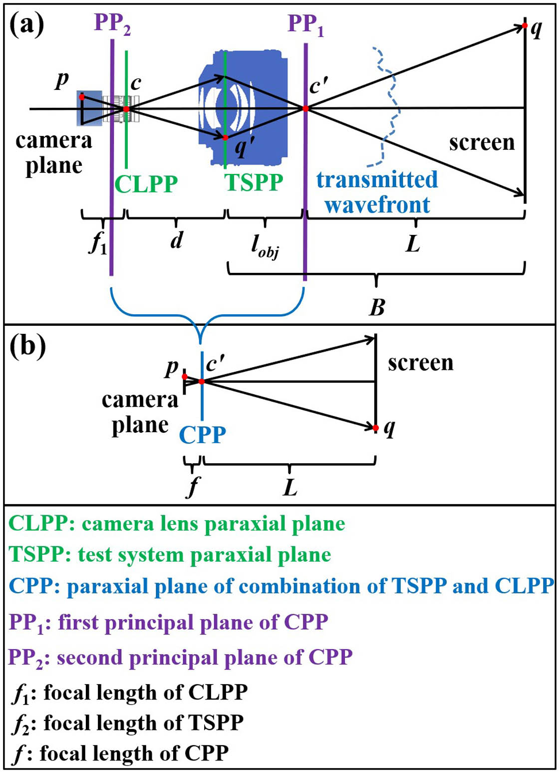
The optical path of our method is shown in Fig. 1(a), comprising a screen, a camera, and the test multilens optical system (shown as an SLR camera lens). Computer-generated fringe patterns are sequentially displayed on the screen. The camera captures the deflection images of the displayed fringe patterns via the test multilens optical system. Light is assumed to be emitted from the camera plane. The camera is modeled by the usual pinhole. $c$ is the camera optical center. A light ray from the pixel point $p$ on the camera plane will finally hit the point $q$ on the screen.

Figure 1.Schematic of our method. (a) Layout of the setup; (b) the part from PP₁ to PP₂ is squeezed into a new paraxial plane, CPP, which plays the role of the camera lens in (b).

We use two paraxial planes to represent the camera lens and the test multilens optical system; they are noted as the camera lens paraxial plane (CLPP) and the test system paraxial plane (TSPP) in Fig. 1(a), respectively. We can consider all the refractions in the test multilens optical system as occurring on TSPP. The focal lengths of the CLPP and TSPP are $f_{1}$ and $f_{2}$ , and $d$ is the distance between them. Always, $d$ is larger than $f_{2}$ . So, light rays are not parallel after passing via the TSPP. All light rays will focus twice at the optical center ( $c$ ) and another point ( $c^{'}$ ) when $d > f_{2}$ .

Furthermore, we use a new combined paraxial plane (CPP), to represent the combination of the TSPP and CLPP, as shown in Fig. 1(b). We can treat refractions on all the transparent phase elements as caused on the CPP. $c^{'}$ is the optical center of the CPP.

In Fig. 1, ${PP}_{1}$ and ${PP}_{2}$ are the first principal plane and second principal plane of the CPP. $l_{obj}$ is the distance between ${PP}_{1}$ and the TSPP. $L$ is the distance between the screen and ${PP}_{1}$ . The CPP can be treated as coming from squeezing the part in Fig. 1(a) from ${PP}_{1}$ to ${PP}_{2}$ .

If the measurement setup is ideally aligned like interferometry, the gradients vector, $g$ , of the transmitted wavefront is represented as $g = \frac{x_{2} - x_{1}}{B},$ (1)where $B$ is the distance between the TSPP and the screen; $x_{1}$ and $x_{2}$ are the coordinates of the light rays on the TSPP and the screen, respectively. From Eq. (1), the wavefront can be obtained by numerical integration^[1,12,13]. The solutions of parameters $x_{2}$ , $B$ , and $x_{1}$ in Eq. (1) are discussed in Sections 2.2, 2.3, and 2.4, respectively.

However, in the actual measurement setup, equipment usually cannot align ideally. Misalignments will bring systematic errors to the wavefront. The calculated wavefront $W$ can be written as the following equation: $W = f_{int 2} (g) = W_{T} + W_{e} = W_{a} + W_{s} + W_{e},$ (2)in which $f_{int 2} (\cdot)$ stands for a 2D integration function; $W_{T}$ is the actual transmitted wavefront, composed of rotationally symmetric part $W_{s}$ and rotationally asymmetric part $W_{a}$ . $W_{e}$ is the systematic error contributed primarily from the misalignments such as decentration, tile, and noncoaxial condition. We must remove $W_{e}$ and $W_{s}$ from $W$ . A relevant solution will be discussed in Section 2.5.

2.1. Calibration strategy of $f$ and $L$

From the perspective of Fig. 1(b), the focal length $f$ , of the CPP, and the distance $L$ , between the ${PP}_{1}$ and the screen can be calibrated. Figure 2 shows the schematic of our calibration strategy. The screen will be moved to different positions with respect to the camera. For each position, the screen displays the same $N$ phase-shifted fringe patterns in the $x$ and $y$ directions. The camera captures the displayed fringe images via the test multilens optical system.

Figure 2.Schematic of calibration strategy in our method.

Then, the wrapped phases in the $x$ and $y$ directions can be calculated using multistep phase-shifting^[14,15] techniques. Pixel points whose values of the wrapped phases equal to $π$ are extracted as the feature points. The 2D world coordinates on the screen can be calculated by these feature points.

Finally, multiple groups of 2D world coordinates are obtained. The focal length $f$ of the CPP can be calibrated by Zhang’s approach^[16]. $L$ is the z-component of the translation vector of the screen.

When calibrating, the screen must be put behind $c^{'}$ . We will prove it in Section 4.1.

2.2. Solution of $x_{2}$

As to phase measuring deflectometry^[17–19], the phase $φ$ in the captured image is a linear measure for the screen coordinates. $x_{2}$ can be expressed as $x_{2} = R \cdot \frac{T u_{s}}{2 π} φ + T,$ (3)where $φ$ is the phase of the fringe; $u_{s}$ is the pixel size of the screen; $T$ is the period of fringes on the screen; $R$ is the rotation matrix of the screen; and $T$ is the translation vector of the screen in $x$ and $y$ directions. The z-component in $φ$ and $T$ is 0.

The phase $φ$ is always coded with the well-known multistep phase-shifting^[14,15] techniques. The screen displays $N$ fringe patterns in the $x$ and $y$ directions, each of which is shifted by $2 π / N$ . Then, the phase can be separately calculated from the $N$ intensities in every pixel. The obtained phase values are always wrapped within $[- π, π]$ . To calculate the gradients using phase values, these wrapped phases must be unwrapped^[20,21].

2.3. Solution of $B$

When $f$ is calibrated using the method in Section 2.1, the distance $d$ between the CLPP and TSPP can be obtained. Since the CPP is composed of two paraxial planes (CLPP and TSPP), its focal length $f$ can be written as Eq. (4)^[22], $f = \frac{f_{1} f_{2}}{Δ},$ (4)where $Δ$ is the optical interval, and can be expressed as Eq. (5), $Δ = d - f_{1} - f_{2} .$ (5)

From Eqs. (4) and (5), $d$ can be written as Eq. (6), $d = \frac{f_{1} f_{2}}{f} + f_{1} + f_{2} .$ (6)

When $d$ is obtained, imaging characters of the CPP are ascertained. From Fig. 1(a), $B$ can be calculated using the following equation: $B = l_{obj} + L,$ (7)in which $L$ can be obtained with the calibration strategy in Section 2.1; $l_{obj}$ can be expressed as^[22] $l_{obj} = f_{2} + x_{F} + f,$ (8)in which $x_{F}$ is the distance from the first focal point of the TSPP to the first principal plane of CPP. $x_{F}$ can be calculated using Eq. (9)^[22], $x_{F} = \frac{f_{2}^{2}}{Δ} .$ (9)

Combining Eqs. (5 )–(9), $B$ can be finally written as Eq. (10), $B = \frac{f_{2} f}{f_{1}} + f_{2} + f + L .$ (10)

2.4. Solution of $x_{1}$

When the measurement setup is ideally aligned, $x_{1}$ can be calculated using the camera’s internal parameters. $x_{1}$ can be expressed as $x_{1} = d (\frac{u_{c}}{f_{1}} x_{c} - δ_{t}) / δ_{r},$ (11)in which $u_{c}$ is the pixel size of the camera plane; $x_{c}$ is the coordinates on the camera plane; $δ_{t}$ and $δ_{r}$ are the tangential distortion and radial distortion, which could be obtained by an additional calibration of the camera^[16].

2.5. Removal of systematic errors

To remove the systematic errors $W_{e}$ and rotationally symmetric part $W_{s}$ , we will conduct an $N$ -rotation test^[23,24]. The test multilens optical system will be measured at $N$ angular positions, equally spaced with respect to the optical axis. Each measurement result at the angular position with the angle of $2 π / N$ can be written as Eq. (12), ${\begin{cases} W^{θ} = W_{a}^{θ} + W_{s} + W_{e} \\ W^{θ + \frac{2 π}{N}} = W_{a}^{θ + \frac{2 π}{N}} + W_{s} + W_{e} \\ ⋮ \\ W^{θ + \frac{2 π}{N} (N - 2)} = W_{a}^{θ + \frac{2 π}{N} (N - 2)} + W_{s} + W_{e} \\ W^{θ + \frac{2 π}{N} (N - 1)} = W_{a}^{θ + \frac{2 π}{N} (N - 1)} + W_{s} + W_{e} \end{cases},$ (12)in which $θ$ is the first angular position. $W_{s}$ and $W_{e}$ will remain unchanged when the test multilens optical system is rotated. The average result of the $N$ -rotation test^[23,24] is the sum of $W_{s}$ and $W_{e}$ ; this relationship can be expressed as Eq. (13), $\bar{W} = \frac{1}{N} \sum_{k = 0}^{N - 1} W^{θ + k \frac{2 π}{N}} = W_{s} + W_{e} .$ (13)

In the end, we can now summarize our method. Rotationally asymmetric wavefront $W_{a}$ of the test multilens optical system can be calculated with Eq. (14), $W_{a} = W - \bar{W},$ (14)in which, by combining Eqs. (1), (2), (3), (10), and (11), $W$ and $\bar{W}$ can be obtained using the following equations: $W = f_{int 2} (\frac{R \cdot \frac{T u_{s}}{2 π} φ + T - (\frac{f_{1} f_{2}}{f} + f_{1} + f_{2}) \cdot (\frac{u_{c}}{f_{1}} x_{c} - δ_{t}) / δ_{r}}{\frac{f_{2} f}{f_{1}} + f_{2} + f + L}),$ (15) $\bar{W} = \frac{1}{N} \sum_{k = 0}^{N - 1} W^{θ + k \frac{2 π}{N}} .$ (16)

3. Simulation

In this section, we simulate the wavefront reconstruction process. The simulated wavefront of the multilens optical system was expressed as 0.1 × amount of peaks (300) (unit: mm), as shown in Fig. 3(a).

Figure 3.Simulation of wavefront reconstruction. (a) Simulated wavefront of the multilens optical system; (b) schematic of the simulated measurement setup. (c)–(g) Results when the screen was expressed as (c) z = 0.1x + 0.2y + 1000, (d) z = 0.1x + 0.2y + 2000, (e) z = 0.1x + 0.2y + 8000, (f) z = 0.3x + 0.3y + 2000, and (g) z = 0.4x + 0.4y + 2000; (h) errors between (a) and (e).

Figure 3(b) is the schematic of the simulated measurement setup. The focal lengths of the CLPP and TSPP were 20 and 60 mm. The distance $d$ from the CLPP to the TSPP was 200 mm. Since $d > f_{2}$ , the transmitted wavefront on TSPP would attach a spherical wave, as shown in Fig. 3(b). Figures 3(c)–3(g) are the restored wavefronts with different screen equations. Figure 3(h) is the error map obtained by subtracting Fig. 3(e) from Fig. 3(a). Figure 3(h) is just the rotationally symmetric part $W_{s}$ , which had been removed from Fig. 3(a) by our method.

From this simulation, we can draw these conclusions. 1.Our method can effectively restore the rotationally asymmetric wavefront $W_{a}$ [by comparing Figs. 3(a) and 3(e)].2.The measuring accuracy will be improved with the increase of the distance between the TSPP and screen [by comparing Figs. 3(c)–3(e)].3.The impact of misalignments in moderation can be negligible in our method [by comparing Figs. 3(d), 3(f), and 3(g)].

4. Experiment

Experiments were conducted to test the performance of our method. A measuring system was developed, including a CCD camera (IDS UI-2340SE-M-GL) and an LCD screen (ASUS MB169B+) with the diagonal length 396.24 mm and the resolution of $1920 pixels \times 1080 pixels$ . The camera resolution was set at $1360 pixels \times 1024 pixels$ . Pixel sizes of the screen and camara were 0.179 mm and 4.65 µm. The focal length of the camera lens was 25 mm. The screen displayed monochromatic red fringes to avoid the effect of chromatic aberration. The wavefront was finally integrated using the Southwell model^[25].

To calculate the unwrapped phase, the three-frequency temporal phase unwrapping^[26,27] method was used. The screen displayed sequentially three groups of phase-shifting fringe patterns with different frequencies ( $f_{l} = 1$ , $f_{m}$ and $f_{h}$ varied with different test objects). The phases at the group with the lowest frequency were always absolute and unwrapped (because $f_{l} = 1$ ) and can be used to guide the unwrapping of the middle-frequency fringes. Finally, high-frequency unwrapped phases were obtained with the guide of the middle-frequency unwrapped phases.

All the test multilens optical systems will be measured at five equally spaced angular positions rotating around the optical axis. These are the positions with the angle of 0°, 72°, 144°, 216°, and 288°, respectively.

4.1. Collimator

A commercial collimator was first selected as the test multilens optical system, where the focal length is 550 mm. Figure 4 shows the whole measurement process.

Figure 4.Measurement process. (a) Measurement setup and the test collimator; (b) pictures acquired when using the temporal phase unwrapping.

Figure 5 shows the test results. Because the rotation accuracy was limited, we removed the first eight Zernike terms. Figures 5(a)–5(e) are the wavefronts at the angular positions with the angle of 0°, 72°, 144°, 216°, and 288°. Figure 5(e) is the interferometry result at 288°.

Figure 5.Test results (the first eight Zernike terms removed). (a)–(e) Wavefronts at the positions with the angles of 0°, 72°, 144°, 216°, and 288°; (f) interferometry result at 288°.

In Figs. 5(a)–5(e), the wavefront maps at the angular positions with different rotation angles are consistent and rotate equally around the optical axis with 72° intervals. In terms of distribution and amplitude (RMS), the results using our proposed method are consistent with the interferometry result.

Moreover, the key aspect of the calibration in Section 2.1, i.e., placing the screen behind $c^{'}$ , was verified. We detected the position $c^{'}$ in advance, and $L$ was calibrated twice when the screen was placed behind and in front of $c^{'}$ . Finally, as shown in Fig. 6(a), L was calibrated as 284.43 mm when the screen was behind $c^{'}$ , which was consistent with the previous detection. However, when the screen was placed in front of $c^{'}$ , an incorrect value of $L = 713.80 mm$ was calibrated, as shown in Fig. 6(b). This can be explained by the simplified imaging model of the double calibration, as shown in Figs. 6(c) and 6(d). When the screen was behind $c^{'}$ , the calibration process was calibrating a pinhole camera, which had a focal length of $f$ . However, when the screen was in front of $c^{'}$ , the camera model was not a common pinhole, without even an optical center. Therefore, when the screen is in front of $c^{'}$ , the incorrect values of $L$ and $f$ are calibrated.

Figure 6.Devices and simplified imaging models of the double calibration when the screen was put (a), (c) behind and (b), (d) in front of c′.

4.2. SLR prime lens

Another commercial optical system was selected to be the second test object: an F/1.8 Nikon Nikkor SLR prime lens, comprising six sublenses, with a focal length of 50 mm and total length of 39 mm. The whole measurement process is shown in Fig. 7.

Figure 7.Measurement process. (a) Measurement setup and the test SLR prime lens; (b) pictures acquired when using the temporal phase unwrapping.

Figure 8 shows the results of our method and interferometric test. Also, due to the limited rotation accuracy, the first eight Zernike terms were removed. The test results show an obvious secondary coma remains in the wavefronts. Wavefront maps at the angular positions with different rotation angles are still consistent, and rotate equally around the optical axis with 72° intervals. Results prove that the measurement accuracy is comparable with interferometric test. Certain blurred spots in Fig. 8 were attributed to the dust on the lens surface.

Figure 8.Test results (the first eight Zernike terms removed). (a)–(e) Wavefronts at the positions with the angles of 0°, 72°, 144°, 216°, and 288°; (f) interferometry result at 288°.

4.3. SLR zoom lens

In the last experiment, we selected an SLR zoom lens as the test multilens optical system: Nikon Nikkor SLR zoom lens, 18–55 mm focal length, comprising 12 sublenses, as shown in Fig. 9. The blue parts in Fig. 9 show the aspherical lens elements. The focal length of this test SLR zoom lens was sequentially set to 18 mm and 55 mm. Two measurements under different focal lengths were conducted to confirm this method. Figure 10 shows the results (the first eight Zernike terms removed).

Figure 9.Diagram of the internal sublenses in the test SLR zoom lens.

Figure 10.Test results (the first eight Zernike terms removed). (a)–(e) Wavefronts at the angular positions with five rotation angles (0°, 72°, 144°, 216°, and 288°) under 18 mm focal length; (f)–(j) wavefronts at the angular positions with five rotation angles (0°, 72°, 144°, 216°, and 288°) under 55 mm focal length.

In Fig. 10, wavefronts at different angular positions under 18 or 55 mm focal length were consistent, and rotated equally around the optical axis with 72° intervals. For the wavefronts with the same angular positions, the maps under 18 and 55 mm focal lengths were still consistent. The results in Fig. 10 confirm the feasibility of this method.

5. Summary

In this study, a wavefront measuring method for an optical system with multiple optics is presented based on PMD. The test multilens optical system and the camera lens are considered as two paraxial planes. Next, a new paraxial plane is used to represent these two separate paraxial planes. We introduced our calibration strategy and mathematical equations to calculate the distance parameters in the measurement setup. The simulations and experiments of three different types of multilens optical systems were performed, which confirm the proposed measuring method. Systematic errors are suppressed using the $N$ -rotation test. The accuracy can be comparable to the interferometric test.

In the past, PMD was primarily used to test a mirror or a single thin lens. The proposed method makes it possible for PMD to test a multilens optical system where the total length can reach 550 mm, similar to a collimator.

References

[1] L. Huang, M. Idir, C. Zuo, A. Asundi. Review of phase measuring deflectometry. Opt. Lasers Eng., 107, 247(2018).

[2] Z. Chen, W. Zhao, Q. Zhang. Wavefront measurement of membrane diffractive lens using line structured light deflectometry. Proc. SPIE, 11617, 116172W(2020).

[3] M. Z. Dominguez, J. Armstrong, P. Su, R. E. Parks, J. H. Burge. SCOTS: a useful tool for specifying and testing optics in slope space. Proc. SPIE, 8493, 84931D(2012).

[4] Y. Liu, X. Su, Q. Zhang. Wavefront measurement based on active deflectometry. Proc. SPIE, 6723, 67232N(2008).

[5] H. A. Canabal, J. Alonso. Automatic wavefront measurement technique using a computer display and a charge-coupled device camera. Opt. Eng., 41, 822(2002).

[6] M. Petz, R. Tutsch. Measurement of optically effective surfaces by imaging of gratings. Proc. SPIE, 5144, 288(2003).

[7] M. Z. Dominguez, L. Wang, P. Su, R. E. Parks, J. H. Burge. Software configurable optical test system for refractive optics. Proc. SPIE, 8011, 80116Q(2011).

[8] L. Jiang, X. Zhang, F. Fang, X. Liu, L. Zhu. Wavefront aberration metrology based on transmitted fringe deflectometry. Appl. Opt., 56, 7396(2017).

[9] P. Su, M. Khreishi, T. Su, R. Huang, M. Z. Dominquez, A. V. Maldonado, G. P. Butel, Y. Wang, R. E. Parks, J. H. Burge. Aspheric and freeform surfaces metrology with software configurable optical test system: a computerized reverse Hartmann test. Opt. Eng., 53, 031305(2014).

[10] R. Huang, P. Su, J. H. Burge, L. Huang, M. Idir. High-accuracy aspheric x-ray mirror metrology using software configurable optical test system deflectometry. Opt. Eng., 54, 084103(2015).

[11] P. Su, S. Wang, M. Khreishi, Y. Wang, T. Su, P. Zhou, R. E. Parks, K. Law, M. Rascon, T. Zobrist, H. Martin, J. H. Burge. SCOTS: a reverse Hartmann test with high dynamic range for giant Magellan telescope primary mirror segments. Proc. SPIE, 8450, 84500W(2012).

[12] L. Huang, A. Asundi. Improvement of least-squares integration method with iterative compensations in fringe reflectometry. Appl. Opt., 51, 7459(2012).

[13] H. Guang, Y. Wang, L. Zhang, L. Li, M. Li, L. Ji. Enhancing wavefront estimation accuracy by using higher-order iterative compensations in the Southwell configuration. Appl. Opt., 56, 2060(2017).

[14] Y. Surrel. Design of algorithms for phase measurements by the use of phase stepping. Appl. Opt., 35, 51(1996).

[15] C. Zuo, S. Feng, L. Huang, T. Tao, W. Yin, Q. Chen. Phase shifting algorithms for fringe projection profilometry: a review. Opt. Lasers Eng., 109, 23(2018).

[16] Z. Zhang. A flexible new technique for camera calibration. IEEE Trans. Pattern Anal., 22, 1330(2000).

[17] M. C. Knauer, J. Kaminski, G. Hausler. Phase measuring deflectometry: a new approach to measure specular free-form surfaces. Proc. SPIE, 5457, 366(2004).

[18] J. H. Massig. Measurement of phase objects by simple means. Appl. Opt., 38, 4103(1999).

[19] C. Faber, E. Olesch, R. Krobot, G. Husler. Deflectometry challenges interferometry: the competition gets tougher!. Proc. SPIE, 8493, 84930R(2012).

[20] D. C. Ghiglia, M. D. Pritt. Two-Dimensional Phase Unwrapping: Theory, Algorithms, and Software(1998).

[21] J. Tian, X. Peng, X. Zhao. A generalized temporal phase unwrapping algorithm for three-dimensional profilometry. Opt. Lasers Eng., 46, 336(2008).

[22] P. Banerjee, T. C. Poon. Principles of Applied Optics(2015).

[23] W. Song, F. Wu, X. Hou. Method to test rotationally asymmetric surface deviation with high accuracy. Appl. Opt., 51, 5567(2012).

[24] C. J. Evans, R. N. Kestner. Test optics error removal. Appl. Opt., 35, 1015(1996).

[25] W. H. Southwell. Wave-front estimation from wave-front slope measurements. J. Opt. Soc. Am., 70, 998(1980).

[26] H. O. Saldner, J. M. Huntley. Temporal phase unwrapping: application to surface profiling of discontinuous objects. Appl. Opt., 36, 2770(1997).

[27] C. Zuo, L. Huang, M. Zhang, Q. Chen, A. Asundi. Temporal phase unwrapping algorithms for fringe projection profilometry: a comparative review. Opt. Lasers Eng., 85, 84(2016).