• High Power Laser Science and Engineering
  • Vol. 6, Issue 2, 02000e35 (2018)
L. Van Box Som1、2、3、*, é. Falize1、3, M. Koenig4、5、6, Y. Sakawa7, B. Albertazzi4、5, P. Barroso8, J.-M. Bonnet-Bidaud3, C. Busschaert1, A. Ciardi2, Y. Hara7, N. Katsuki9, R. Kumar7, F. Lefevre4、5, C. Michaut10, Th. Michel4、5, T. Miura9, T. Morita9, M. Mouchet10, G. Rigon4、5, T. Sano7, S. Shiiba9, H. Shimogawara7, and S. Tomiya11
Author Affiliations
  • 1CEA-DAM-DIF, F-91297 Arpajon, France
  • 2LERMA, Sorbonne Université, Observatoire de Paris, Université PSL, CNRS, F-75005 Paris, France
  • 3CEA Saclay, DSM/Irfu/Service d’Astrophysique, F-91191 Gif-sur-Yvette, France
  • 4LULI - CNRS, Ecole Polytechnique, CEA: Université Paris-Saclay
  • 5UPMC Univ Paris 06: Sorbonne Université - F-91128 Palaiseau Cedex, France
  • 6Graduate School of Engineering, Osaka University, Suita, Osaka 565-0871, Japan
  • 7Institute of Laser Engineering, Osaka University, Suita, Osaka 565-0871, Japan
  • 8GEPI, Observatoire de Paris, PSL Research University, CNRS, Université Paris Diderot, Sorbonne Paris Cité, F-75014 Paris, France
  • 9Faculty of Engineering Sciences, Kyushu University, 6-1 Kasuga-Koen, Kasuga, Fukuoka 816-8580, Japan
  • 100LUTH, Observatoire de Paris, PSL Research University, CNRS, Université Paris Diderot, Sorbonne Paris Cité, F-92195 Meudon, France
  • 11Aoyama Gakuin University, Japan
  • show less
    DOI: 10.1017/hpl.2018.32 Cite this Article Set citation alerts
    L. Van Box Som, é. Falize, M. Koenig, Y. Sakawa, B. Albertazzi, P. Barroso, J.-M. Bonnet-Bidaud, C. Busschaert, A. Ciardi, Y. Hara, N. Katsuki, R. Kumar, F. Lefevre, C. Michaut, Th. Michel, T. Miura, T. Morita, M. Mouchet, G. Rigon, T. Sano, S. Shiiba, H. Shimogawara, S. Tomiya. Laboratory radiative accretion shocks on GEKKO XII laser facility for POLAR project[J]. High Power Laser Science and Engineering, 2018, 6(2): 02000e35 Copy Citation Text show less
    Target’s schematic. The laser comes from the right and it interacts with the pusher. A plasma is created due to the interaction between the laser and the pusher. This supersonic plasma expands in the vacuum and impacts an obstacle. This leads to the creation of a reverse shock.
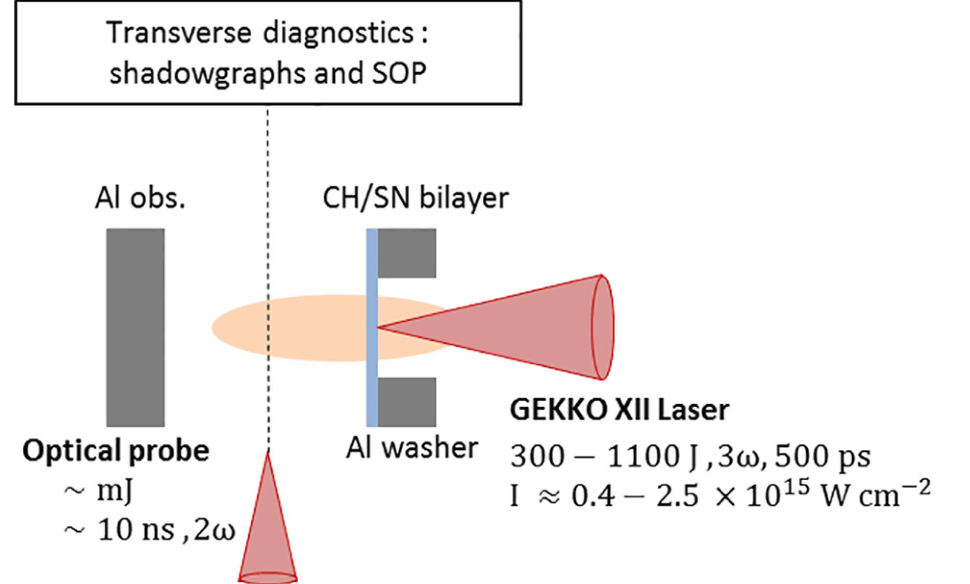
    Fig. 1. Target’s schematic. The laser comes from the right and it interacts with the pusher. A plasma is created due to the interaction between the laser and the pusher. This supersonic plasma expands in the vacuum and impacts an obstacle. This leads to the creation of a reverse shock.
    Spatial evolution of the density as a function of time extracted from 1D simulation performed with FCI2 code. The position axis is horizontal, whereas the time evolution is the vertical axis. The laser deposits 600 J on the target, and it comes from the right. The distance to the obstacle is 3.5 mm.
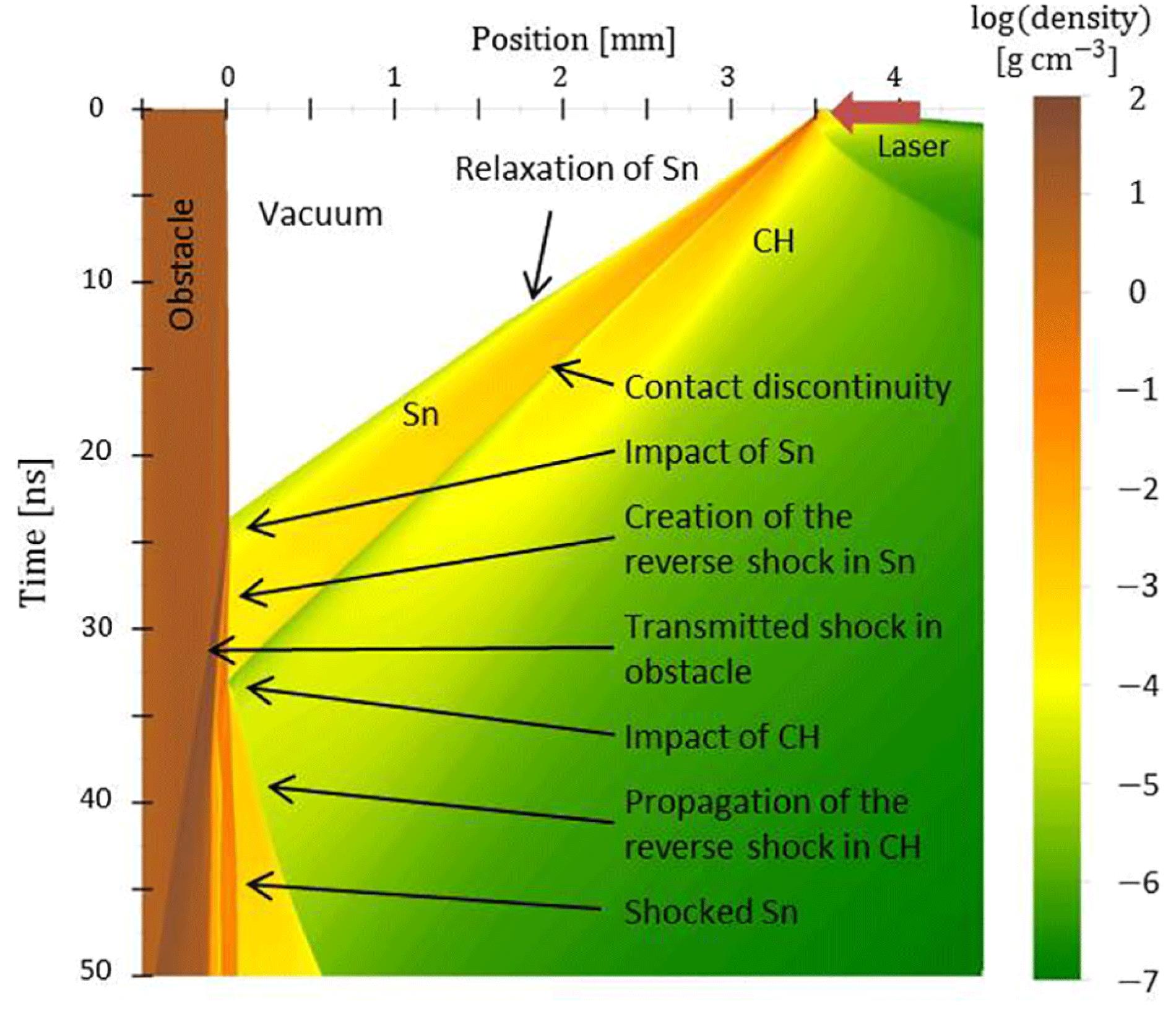
    Fig. 2. Spatial evolution of the density as a function of time extracted from 1D simulation performed with FCI2 code. The position axis is horizontal, whereas the time evolution is the vertical axis. The laser deposits 600 J on the target, and it comes from the right. The distance to the obstacle is 3.5 mm.
    2D snapshot shadowgraphy obtained at 13 ns after the laser drive of the incident plasma flow.
    Fig. 3. 2D snapshot shadowgraphy obtained at 13 ns after the laser drive of the incident plasma flow.
    (a) Density and (b) temperature maps of the incident flow around 10 ns before the collision extracted from 2D FCI2 simulation.
    Fig. 4. (a) Density and (b) temperature maps of the incident flow around 10 ns before the collision extracted from 2D FCI2 simulation.
    (a) 2D snapshot interferometry obtained at 11 ns after the laser drive of the incident flow compared with (b) the associated electronic density. The experimental electronic density is compared to iso-density curves at , and extracted from 2D simulations (black lines).
    Fig. 5. (a) 2D snapshot interferometry obtained at 11 ns after the laser drive of the incident flow compared with (b) the associated electronic density. The experimental electronic density is compared to iso-density curves at , and extracted from 2D simulations (black lines).
    1D shadowgraphy used to determine the velocity of the incident flow. The plasma created by the laser comes from the right. The position is relative to the obstacle position, whereas the vertical axis presents the time evolution.
    Fig. 6. 1D shadowgraphy used to determine the velocity of the incident flow. The plasma created by the laser comes from the right. The position is relative to the obstacle position, whereas the vertical axis presents the time evolution.
    1D self-emission (SOP). The plasma created by the laser comes from the right. The position is relative to the obstacle position, whereas the vertical axis presents the time evolution. The CH flow position (white dotted line), the reverse shock position (white line) and the 10 eV iso-contour (black line) extracted from 2D simulations are added.
    Fig. 7. 1D self-emission (SOP). The plasma created by the laser comes from the right. The position is relative to the obstacle position, whereas the vertical axis presents the time evolution. The CH flow position (white dotted line), the reverse shock position (white line) and the 10 eV iso-contour (black line) extracted from 2D simulations are added.
    Experimental velocities of the incident flow as functions of the laser energy extracted from the 1D shadowgraphies (blue squares) and from the 1D SOP (red points). They are compared to velocities extracted from 2D simulations: velocities of the iso-temperature curve at 5 eV (black triangles) and velocities of the iso-density curve at density (black diamonds).
    Fig. 8. Experimental velocities of the incident flow as functions of the laser energy extracted from the 1D shadowgraphies (blue squares) and from the 1D SOP (red points). They are compared to velocities extracted from 2D simulations: velocities of the iso-temperature curve at 5 eV (black triangles) and velocities of the iso-density curve at density (black diamonds).
    Density and temperature maps of the incident flow extracted from 2D numerical simulation around (a) 5 ns and (b) 20 ns after the collision. Just after the collision, the reverse shock is not propagated, whereas a radiative flash is clearly visible in the impact zone. Around 20 ns after the collision, the reverse shock has caught up with the radiative structure.
    Fig. 9. Density and temperature maps of the incident flow extracted from 2D numerical simulation around (a) 5 ns and (b) 20 ns after the collision. Just after the collision, the reverse shock is not propagated, whereas a radiative flash is clearly visible in the impact zone. Around 20 ns after the collision, the reverse shock has caught up with the radiative structure.
    Velocities and cooling parameters in the POLAR project as a function of the laser power. Simulations are presented by dotted black lines. Experimental results obtained with intermediate laser facilities are displayed by coloured dots. The results obtained with GEKKO XII are presented by blue dots.
    Fig. 10. Velocities and cooling parameters in the POLAR project as a function of the laser power. Simulations are presented by dotted black lines. Experimental results obtained with intermediate laser facilities are displayed by coloured dots. The results obtained with GEKKO XII are presented by blue dots.
    Obstacle distance (mm)AM
    Laser energy (J)Herculis
    ()
    ()
    (eV)
    Table 1. Similarity properties of four typical shots at different laser energies and different distances from the obstacle. Values are extracted from the 2D simulations performed with the FCI2 code.
    L. Van Box Som, é. Falize, M. Koenig, Y. Sakawa, B. Albertazzi, P. Barroso, J.-M. Bonnet-Bidaud, C. Busschaert, A. Ciardi, Y. Hara, N. Katsuki, R. Kumar, F. Lefevre, C. Michaut, Th. Michel, T. Miura, T. Morita, M. Mouchet, G. Rigon, T. Sano, S. Shiiba, H. Shimogawara, S. Tomiya. Laboratory radiative accretion shocks on GEKKO XII laser facility for POLAR project[J]. High Power Laser Science and Engineering, 2018, 6(2): 02000e35
    Download Citation