Evaluation of the mirror surface figure error based on the slope of the root-mean square

Fuguo Wang; Qichang An; Limin Zhang

doi:10.3788/COL201513.S22202

Abstract

The slope of the root-mean square (RMS) can be applied to evaluate mid-spatial frequency mirror surface errors for larger-aperture mirrors. In this paper, the slope RMS is analyzed from three different perspectives. First, the relationship between the slope RMS and the basis polynomials is discussed, and the mathematical relationship between the slope RMS and the standard orthogonal basis is obtained. Second, the slope RMS is analyzed by applying the Wiener process, with the results indicating that the ideal mirror surface error obeys the Gauss distribution law. Then, a power spectrum analysis method based on the slope RMS is proposed. Finally, the method is used to analyze the Thirty Meter Telescope tertiary mirror surface figure.

A variety of methods exist to evaluate the surface figure error of reflective mirrors. As a traditional evaluation method, the root-mean square (RMS) is typically used to describe the surface figure error of small-aperture mirrors. Because the size of the grinding tools and the size of the optical components are similar, it can be applied to describe the simplest optical characteristics^[1,2].

However, for large-aperture reflective mirrors, this evaluation method faces several limitations. First, the small size of the grinding tools that are employed to polish the large-aperture mirror will produce sub-aperture-scale and mid-spatial frequencies, especially for aspheric surfaces and free surfaces. Particularly, the grinding smoothness depends on a uniform distribution caused by the tools and the holding pressure time. Second, a multi-point support is always used for large-aperture mirrors. As the number of support points increases, the mirrors will become more prone to mid-spatial frequencies. These mid-spatial frequencies produced by fringe irregularities are several times smaller than the optical element aperture, but larger than the surface’s precision structure, i.e., the mirror surface roughness^[3,4].

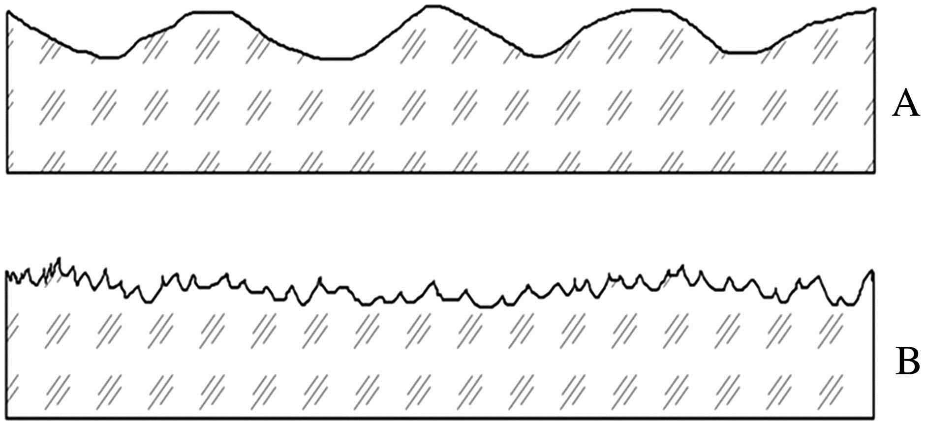
For different spatial frequency mirror surface figure errors, different evaluation methods produce different results. Figure 1 shows a schematic illustration of two different optical surface figure errors. The optical surface of Mirror A exhibits low-frequency errors, while the optical surface of Mirror B shows high-frequency errors. When using the traditional RMS optical surface evaluation method, the RMS value is relatively large for Mirror A, and relatively small for Mirror B, and consequently, Mirror A is unqualified, and Mirror B is qualified. However, Mirror A mainly exhibits low-frequency errors, which can be easily corrected by applying adaptive optics, whereas the high-frequency errors of Mirror B are difficult to correct by adaptive optics. Therefore, the RMS evaluation method has its limitations for large-aperture mirrors. In contrast, if using the slope of the RMS to evaluate the mirror surface error, the slope RMS value obtained for Mirror A is small, and the slope RMS obtained for Mirror B is large. Thus, Mirror A is qualified, and Mirror B is unqualified^[1–4].

Sign up for Chinese Optics Letters TOC. Get the latest issue of Chinese Optics Letters delivered right to you！Sign up now

Figure 1.Schematic illustration of two different mirror surface figures: (a) with low-frequency errors; (b) with high-frequency errors.

For large-aperture mirrors, the surface figure test and evaluation directly affects the manufacturing accuracy and imaging quality^[5,6]. The RMS test shows obvious shortcomings for evaluating large-aperture mirrors. In recent years, some researchers therefore proposed using the slope RMS to evaluate the mirror surface error in the time domain. Although it can control rigid body displacements and reflect a wide range of roughnesses^[7,8], for small scale shakes, there will be dramatic fluctuations. Therefore, an analysis based on the frequency domain is necessary.

Low-order wavefront errors are always fitted by basis polynomials. More precisely, the wavefront error can be described by discrete index basis polynomials $Φ (m, n) = \sum a_{u v} W_{u v} (m, n),$ (1)where $a_{u v}$ is the basis fitting coefficient, $Φ (m, n)$ is the wave front error, $a (m, n)$ is the coefficient, and $W_{u v} (m, n)$ is the basal function.

For an $N \times N$ sampling aperture, $W_{u v} (m, n)$ can be expressed by $W_{u v} (m, n) = \frac{1}{N \times N} \exp [\frac{2 π j}{N} (u m + v n)],$ (2)where $W_{u v} (m, n)$ is the wave aberration. For convenience, only the imaginary component is considered in the one-dimensional case, resulting in a standard sine polynomial. If the wavefront error energy is constant, the RMS cannot be used to comprehensively reflect its dynamic performance. Therefore, the slope RMS is applied to address this problem $Φ = A \sin (2 π f x),$ (3) ${(\nabla Φ)}^{2} = {(\nabla A \sin (2 π f x))}^{2} = 4 A^{2} π^{2} f^{2} \cos^{2} (2 π f x) 〈 \nabla Φ^{2} 〉 = \frac{2 A^{2} π f \int_{0}^{1 / f} \cos^{2} (2 π f x) 2 π f d x}{1 / f} .$ (4)where $f$ is the spatial frequency, $A$ is the error of the amplitude. For the standard sine polynomial in Eq. (3), the wavefront error is constant, i.e., ${RMS}_{φ} = A$ . Its slope RMS can be expressed by $Φ = \sqrt{2} A \sin (2 π f x),$ (5) $slop RMS = \sqrt{2} π f A .$ (6)It is generally assumed that the wavefront error is a linear combination of two standard sine polynomials, as illustrated by Fig. 2, and its slope RMS can be expressed as $Φ = α \sqrt{2} A \sin (2 π f x) + β Φ = \sqrt{2} A \sin (2 π 2 f x),$ (7) $slope {RMS}^{2} = {(\sqrt{2 a^{2} + 8 β^{2}} π A f)}^{2} = α^{2} 2 f^{2} A^{2} + β^{2} 8 f^{2} A^{2} .$ (8)

Figure 2.Illustration of the multiplied wavefront error.

An extension of this construction to rank $N$ yields $slope {RMS}^{2} = \sum_{1}^{N} c_{i}^{2} slope {RMS}_{i}^{2} .$ (9)This suggests that, if the wavefront error is expressed by a standard orthogonal basis such as a standard sine polynomial, every item’s slope RMS can be calculated individually, with the total slope RMS then obtained by summation. In actual engineering applications, some item’s slope RMS can be first calculated as well, and then the total slope RMS can be obtained.

For the surface figure of a reflective mirror, even for an absolutely ideal surface, the measurement instrument will produce an unavoidable error that will affect the mirror surface data; on the other hand, because of other uncontrollable factors (pressure disc jitter, thermal motion of magnetron fluid particles, and random motion of beam particles), the actual surface figure will contain irregular fluctuations after the mirror has been polished.

The mathematical model of the Wiener process was proposed by Einstein to analyze Brownian movement, essentially capturing the irregular movement by using a set of mathematical rules. This Letter will analyze the mirror surface figure by referring to the Wiener process.

According to the basic assumptions of the Wiener process, in the measurement range, the mirror surface slope is zero at the starting point, whereas the surface slope has the following properties: 1.Each coordinate component of the mirror surfaceslope $ω (d_{1}) - ω (u_{1}), ω (d_{2}) - ω (u_{2}) \dots ω (d_{n}) - ω (u_{n})$ is independent. For one of the components, it is denoted as $ω (l)$ , while for arbitrary mutually disjoint regions, it is denoted as $[d_{1}, u_{1}], [d_{2}, u_{2}] \dots [d_{n}, u_{n}]$ .2.The ideal error should be symmetrically distributed, such that $E {w (l)} = 0$ .3.The $w (l + Δ) - w (l)$ distribution does not depend on $l$ . Furthermore, $σ^{2} (Δ) = E {{(w (l + Δ) - w (l))}^{2}}$ exists and is the continuous function of $Δ$ . As a result $Φ (l, λ) = E {e^{i λ w (l)}} = \int_{- \infty}^{+ \infty} e^{i λ x} f (l, x) d x,$ (10) $σ^{2} (l) = E {{[w (l) - w (0)]}^{2}} = E {w^{2} (l)} = \int_{- \infty}^{+ \infty} x^{2} f (l, x) d x,$ (11) where $f (l, x)$ is a probability distribution. Then $σ^{2} (l + s) = E {{[w (l + s) - w (l) + w (l) - w (0)]}^{2}} = E {{[w (l + s) - w (l)]}^{2}} + E {w^{2} (l)} = σ^{2} (s) + σ^{2} (l),$ (12) $σ^{2} (l) = C l (C > 0),$ (13) $Φ (l + s, λ) - Φ (l, λ) = Φ (l, λ) E {e^{i λ (w (s) - w (0))} - 1},$ (14) $e^{i v} \approx 1 + i v - v^{2} / 2 .$ (15)Therefore $\frac{Φ (l + s, λ) - Φ (l, λ)}{s} \approx - \frac{1}{2} λ^{2} Φ (l, λ) C .$ (16)If $s \to 0$ , then $\frac{\partial Φ (l, λ)}{\partial l} = - \frac{1}{2} λ^{2} Φ (l, λ) C,$ (17)since $Φ (0, λ) = 1$ .

We finally obtain $Φ (l, λ) = \int_{- \infty}^{+ \infty} e^{i λ x} \frac{1}{\sqrt{2 π C l}} e^{- \frac{x^{2}}{2 C t}} d x .$ (18)From Eq. (4), it can be concluded that the slope RMS of the ideal mirror surface figure error should obey the Gauss distribution law, and consequentially the slope RMS energy should obey the equipartition law.

Suppose there is a stochastic process ${X (t), t \in T}$ . For every $t$ , the first moment $E [x_{1}]$ and the second moment $E [x_{2}]$ exist. Therefore, we define ${X (t), t \in T}$ as the second-moment process.

Assuming that there is no destruction, the measured mirror surface slope will never be infinite. Since the first moment $E [x_{1}]$ and the second moment $E [x_{2}]$ always exist, the random series describing the mirror surface figure wavefront error is a second-moment process.

Considering the coefficient $R (φ (x + r), φ (x))$ for a second-moment process, by applying the Cauchy–Schwarz Law, we obtain $R^{2} (θ (x + r), θ (x)) = {E {[θ (x + r) θ (x)]}}^{2} \leq E [θ^{2} (x + r)] E [θ^{2} (x)] < + \infty .$ (19)Thus the coefficient $R (θ (x + r), θ (x))$ for the second-moment process always exists, and thereby satisfies the condition for Fourier transformation, i.e., it can be processed to perform a power spectrum analysis. Furthermore, due to its invariability and time-invariance, the expectation can be regarded as a steady-state process.

The power spectrum density (PSD) is defined as $S (w) = \sum_{- \infty}^{+ \infty} R (m) e^{- j w} = \sum_{- \infty}^{+ \infty} E [x (n) x^{*} (n + m)] e^{- j w} .$ (20)For a random series describing the reflective mirror surface wavefront error, its self-correction function can be expressed by $R (r) = {〈 θ (x + r) θ (x) 〉}_{x},$ (21)and the self-power spectrum density is given by $S (\bar{w}) = F (R (r)) = F ({〈 θ (x + r) θ (x) 〉}_{x}) .$ (22)The previous discussion suggests that the system wavefront error is composed of a low-order wavefront error and a high-order noise (with an almost ideal Gauss distribution). Then, by applying the aforementioned methods, the standard Zernike polynomials for describing the coma, astigmatism, and quatrefoil were analyzed, and the results are shown in Figs. 3–5, respectively $S (w) = \sum_{- \infty}^{+ \infty} R (m) e^{- j w} = \sum_{- \infty}^{+ \infty} E [x (n) x^{*} (n + m)] e^{- j w},$ (23) $R (r) = {〈 θ (x + r) θ (x) 〉}_{x},$ (24) $S (\bar{w}) = F (R (r)) = F ({〈 θ (x + r) θ (x) 〉}_{x}) .$ (25)The power spectrum analysis reveals that the energy peaks are shifted to higher frequencies with increasing order of the Zernike polynomials. At the same time, the frequency width also increases. After the data has been normalized, the basic aberration of the actual surface figure power spectrum can be analyzed (Figs. 3–5).

The Thirty Meter Telescope (TMT) is an optical and infrared telescope. Its tertiary mirror is a $3594 mm \times 2536 mm$ elliptical flat mirror with a thickness of 100 mm. Because the TMT primary segment mirror and deformable mirror are able to correct the tertiary mirror surface figure error, if the traditional RMS method is used to evaluate the TMT tertiary mirror surface figure, it cannot generally and objectively reflect the requirements of the tertiary mirror^[9].

Figure 3.Coma power spectrum.

Figure 4.Astigmatism power spectrum.

Figure 5.Quatrefoil power spectrum.

An 18-point support structure is used for the TMT tertiary mirror and the resulting surface figure error is shown in Fig. 6. The error was normalized to a unit circle, as shown in Fig. 7, and its PSD is shown in Fig. 8.

Figure 6.Tertiary mirror surface figure error (tilt removed).

Figure 7.Normalized tertiary mirror surface figure error.

Figure 8.PSD of the TMT tertiary mirror.

Figure 8 indicates that the main deformation of the TMT tertiary mirror is smaller than the coma component (defocus and astigmatism). However, in order to perform an ideal finite-element analysis, the high-frequency contribution is considered to be zero. It is advantageous to differentiate the system aberration by applying the frequency domain analysis method, as well as to evaluate the surface figure error.

For the TMT tertiary mirror surface figure error with removed defocus and astigmation, a slope RMS of 0.98 μrad was obtained. Then, from Eq. (2), the frequency $f_{0} = \frac{slope RMS}{\sqrt{2} π A}$ , which is defined as the system-limiting frequency, can be obtained.

In conclusion, the slope RMS is mathematically analyzed from three different perspectives, some basic characteristics are obtained, and a power spectrum analysis method is proposed. The discrete random series for the Zernike polynomials is analyzed by using the slope RMS method, and the spectrum energy distribution for the Zernike polynomials is obtained. Finally, the TMT tertiary mirror surface figure error is analyzed by applying the slope RMS method, indicating that this method is superior for larger-aperture mirror surface figures.

References

[1] Y. Bi, J. Zhai, J. H. Wu, Q. Hu. Opt. Technol., 35, 10(2009).

[2] D. Wang, H. B. Yang, C. Zh. Chen. Comput. Simul., 24, 298(2007).

[3] P. J. VanZwol, G. Palasantzas, J. Th. M. De Hosson. Appl. Phys. Lett., 91, 144108(2007).

[4] W. Dierking. Proc. IEEE, 38, 1451(2000).

[5] R. Zhelem. Proc. SPIE, 7931, 808310(2011).

[6] A. M. Hvise, J. H. Burge. Proc. SPIE, 6671, 66710A(2007).

[7] Y. CH. Wang, H. Y. Sun, W. Y. Tang, Ch. R. Jiangand, S. Q. Tian. Opt. Precis. Eng., 22, 1606(2014).

[8] K. Huang, F. Fan, H. Gong. Opt. Precis. Eng., 21, 10(2013).

[9] F. G. Wang, Q. Ch. An. Opt. Precis. Eng., 22, 1171(2014).