Propagation of transverse photonic orbital angular momentum through few-mode fiber

Qian Cao; Zhuo Chen; Chong Zhang; Andy Chong; Qiwen Zhan

doi:10.1117/1.AP.5.3.036002

Abstract

Spatiotemporal optical vortex (STOV) pulses can carry transverse orbital angular momentum (OAM) that is perpendicular to the direction of pulse propagation. For a STOV pulse, its spatiotemporal profile can be significantly distorted due to unbalanced dispersive and diffractive phases. This may limit its use in many research applications, where a long interaction length and a tight confinement of the pulse are needed. The first demonstration of STOV pulse propagation through a few-mode optical fiber is presented. Both numerical and experimental analysis on the propagation of STOV pulse through a commercially available SMF-28 standard telecommunication fiber is performed. The spatiotemporal phase feature of the pulse can be well kept after the pulse propagates a few-meter length through the fiber even with bending. Further propagation of the pulse will result in a breakup of its spatiotemporal spiral phase structure due to an excessive amount of modal group delay dispersion. The stable and robust transmission of transverse photonic OAM through optical fiber may open new opportunities for transverse photonic OAM studies in telecommunications, OAM lasers, and nonlinear fiber-optical research.

Keywords

multimode fiber photonic orbital angular momentum spatiotemporal optical vortices

1 Introduction

Since Allen1 published his paper on discovering that higher-order Laguerre–Gaussian beam with a spiral phase wavefront $\exp (i l θ_{x - y})$ carries photons with a longitudinal orbital angular momentum (OAM) in 1992, great success has occurred in the past three decades on utilizing optical vortex beam with OAM in research fields such as optical manipulation,2 optical communication,3 quantum optics,4 superresolution microscopy,5 and many others.6^,7 Very recently, scientists have discovered, both theoretically and experimentally, that photons can also carry a transverse photonic OAM in the form of spatiotemporal optical vortex (STOV) pulses.8^–11 Differing from the vortex beam, the STOV pulse has a spiral phase $\exp (i l θ_{x - t})$ in the spatiotemporal domain ( $x - t$ plane). The STOV pulse, therefore, can carry a transverse photonic OAM of $l ℏ$ per photon.12^–14 Since its discovery, much research has been done in studying STOV pulse, including studying its propagation dynamics,15^,16 developing novel characterization approaches,17^–19 utilizing STOV pulse in spatiotemporal imaging,20 and designing other types of wave packets that also carry transverse photonic OAM.21^–25

STOV pulse has a spatiotemporally coupled field distribution. Under an unbalanced dispersion and diffraction phase, the STOV pulse can be significantly distorted,15^,16 leading to a breakup of the STOV charge and splitting the STOV pulse into multiple lobes in the spatiotemporal domain. This limits the use of the STOV pulse in many applications where a long interaction length and a tight confinement of the pulse are needed. One solution for overcoming this limitation is to generate a STOV pulse in a Bessel form in the spatiotemporal domain so the STOV charge is confined within a tight space-time cross section and the STOV pulse can be nonspreading when it propagates in a dispersive medium.26^,27 However, this Bessel STOV approach requires the pulse to be engineered to accommodate the dispersion relationship of the medium, and the resulting nonspreading propagation distance is still limited by the finite spatial and spectral width of the pulse.

Another approach for achieving a long-distance, stable propagation of the STOV pulse is to use a few-mode optical fiber to guide the STOV pulse. A step-index fiber can support multiple guiding modes if the $V$ -number, defined as $V = k_{0} a \cdot N A$ , is larger than 2.405,28 which forms the fundamental basis for propagating the STOV pulse. Till now, no study on transmitting a STOV pulse through optical fiber or waveguide has been demonstrated. Questions such as how the STOV pulse is going to evolve spatiotemporally after propagating through the fiber, what the maximum transmission length is, and whether it can propagate forever inside the fiber are yet to be explored.

Sign up for Advanced Photonics TOC. Get the latest issue of Advanced Photonics delivered right to you！Sign up now

To answer these questions, we present here what we believe is the first demonstration of STOV pulse propagation through a few-mode optical fiber. We choose a commercially available, standard telecommunication fiber, SMF-28, as our platform to perform all the studies. We implement both numerical and experimental analysis on propagating the STOV pulse through the fiber. The spatiotemporal spiral phase structure of STOV pulses can be kept well for a considerable length of a few meters. Further propagating the pulse inside the fiber will result in a breakup of its phase structure due to an excessive amount of group delay difference. Nevertheless, our experiment achieved a long-distance, stable, and robust transmission of transverse photonic OAM through the fiber. This will bring new opportunities in utilizing transverse photonic OAM in optical telecommunication, building novel transverse OAM lasers, and studying nonlinear fiber optical phenomena that involve transverse OAM.

2 Theoretical Analysis and Numerical Simulations

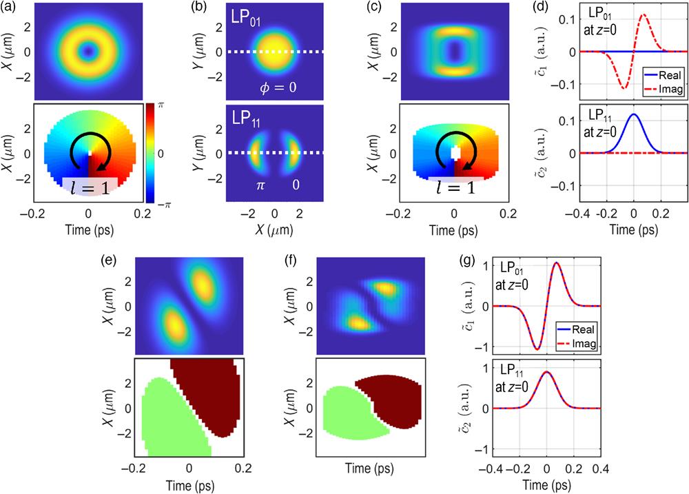
The STOV pulse has an annular intensity profile with a spiral phase of $\exp (i l θ_{x - t})$ in the spatiotemporal ( $x - t$ ) domain. Figure 1(a) shows the spatiotemporal intensity and phase profile of a STOV pulse with a topological charge of $l = + 1$ . The analytical expression for the STOV pulse (including chirped STOV pulse) can be found in Eqs. (6) and (7) in Ref. [15]. As the spatiotemporal phase is whirling inside the pulse, the spatial mode of the STOV pulse varies significantly over time. To transmit it inside the optical fiber, the fiber must support multiple guiding modes. We choose a standard commercially available telecommunication fiber, Corning SMF-28, as our platform to study STOV pulse propagation. SMF-28 has a cutoff wavelength at 1260 nm.29 Assuming that the input STOV pulse is linearly polarized (LP) with a center wavelength of 1030 nm, under weakly guiding approximation, the STOV pulse can be coupled into two LP modes of SMF-28, ${LP}_{01}$ and ${LP}_{11}$ mode. Figure 1(b) plots the spatial intensity profile of ${LP}_{01}$ and ${LP}_{11}$ mode with their spatial phase captioned in the figure. To simplify the calculation process, we choose the field along the horizontal dashed line shown in Fig. 1(b) as the eigen function for the LP modes. An LP STOV pulse can be thus decomposed into the combination of ${LP}_{01}$ and ${LP}_{11}$ mode, written as $E_{STOV} (x, t; z) = \tilde{c_{1}} (t; z) E_{01} (x) + \tilde{c_{2}} (t; z) E_{11} (x),$ (1)where $\tilde{c_{1}} (t; z)$ and $\tilde{c_{2}} (t; z)$ are the complex coefficient for ${LP}_{01}$ and ${LP}_{11}$ mode. $t$ is the localized time coordinate for characterizing the STOV pulse and $z$ is the longitudinal coordinate for the fiber length. $E_{01} (x)$ and $E_{11} (x)$ are the normalized eigen function for ${LP}_{01}$ and ${LP}_{11}$ mode.

Figure 1.Modal decomposition of STOV pulse and focused STOV pulse in LP modes. (a) Spatiotemporal intensity and phase profile of a STOV pulse ( $l = + 1$ ); (b) spatial intensity profile of ${LP}_{01}$ and ${LP}_{11}$ modes in SMF-28; (c) STOV pulse ( $l = + 1$ ) synthesized by LP modes; (d) complex coefficient for LP modes for synthesizing a STOV pulse. (e) spatiotemporal intensity and phase profile of a focused STOV pulse ( $l = + 1$ ); (f) focused STOV pulse ( $l = + 1$ ) synthesized by LP modes; (g) complex coefficient for LP modes for synthesizing a focused STOV pulse.

Figure 1(c) shows the spatiotemporal profile of the STOV pulse with a topological charge of $l = + 1$ synthesized by ${LP}_{01}$ and ${LP}_{11}$ mode. Compared with the STOV pulse in free space [Fig. 1(a)], the STOV pulse in a few-mode fiber is more confined spatially in the $x$ direction due to the waveguide structure. Nevertheless, the spatiotemporal phase feature of the STOV pulse can be kept in this modal decomposition. The complex coefficients $\tilde{c_{1}}$ and $\tilde{c_{2}}$ in Eq. (1) are obtained by calculating the overlapping integral between the STOV pulse and the eigen function. Figure 1(d) plots the real part and the imaginary part of $\tilde{c_{1}}$ and $\tilde{c_{2}}$ over time, respectively. There is a $π / 2$ phase difference between $\tilde{c_{1}}$ and $\tilde{c_{2}}$ .

In the STOV pulses shown in Figs. 1(a) and 1(c), we have assumed that the STOV pulse is already propagating inside the fiber. In practice, a free-space STOV pulse is normally focused into the fiber by an aspherical lens. Figure 1(e) shows the spatiotemporal intensity and phase profile when the STOV pulse is focused. Differing from its free-space form, a focused STOV pulse has two lobes with a $π$ -phase difference between them. Assuming this focused STOV pulse can be perfectly coupled into the fiber, it can be then decomposed into LP modes, as shown in Fig. 1(f). The phase feature is still well kept. Figure 1(g) plots the complex coefficients of the LP modes. Differing from previous modal decomposition, $\tilde{c_{1}}$ and $\tilde{c_{2}}$ are now in phase with each other.

To simulate the STOV pulse propagation inside the fiber, we need to make two assumptions: (1) the STOV pulse is propagating linearly inside the fiber without any loss and (2) there is no cross talk between different LP modes. With these assumptions, the evolution of the STOV pulse is dictated by the propagation constant $β$ , including its dispersion relationship. These parameters can be numerically calculated by solving the paraxial Helmholtz equation. 27 Table 1 lists the calculated effective refractive index $n_{eff}$ , effective group index $n_{g}$ , and the group velocity dispersion (GVD) coefficient $β_{2}$ at 1030 nm. $Δ T$ is the group delay difference between the ${LP}_{01}$ and ${LP}_{11}$ modes. After propagation, 1 m length inside the fiber, ${LP}_{01}$ -mode pulse will lead ${LP}_{11}$ -mode pulse by 170 fs.


Parameter	Brief Description	Mode	Value	Unit
$n_{eff}$	Effective refractive index, $n_{eff} = β / k_{0}$	${LP}_{01}$	1.446191
${LP}_{11}$	1.443798
$n_{g}$	Effective group index, $n_{g} = c / v_{g}$ , $v_{g} = (β_{1})^{- 1} = {(\partial β / \partial ω)}^{- 1}$	${LP}_{01}$	1.463457
${LP}_{11}$	1.463508
$β_{2}$	GVD coefficient, $β_{2} = \partial^{2} β / \partial ω^{2}$	${LP}_{01}$	18.99	${fs}^{2} / mm$
${LP}_{11}$	28.61
$Δ T$	Group delay difference between ${LP}_{01}$ and ${LP}_{11}$		−170	fs/m

Table 1. Propagation parameters for ${LP}_{01}$ and ${LP}_{11}$ modes of SMF-28.

View all Tables

We now perform numerical simulation of the focused STOV pulse propagation in SMF-28 by setting the virtual fiber length at 100, 200, and 300 cm. The STOV pulse has a topological charge of $l = + 1$ . Figure 2(a) shows the results when an unchirped focused STOV pulse is propagating. Due to the GVD and group velocity mismatch (GVM), a focused STOV pulse is distorted during pulse propagations. However, at 100 and 200 cm, the spatiotemporal spiral phase of the STOV pulse is still well preserved, showing a spiral phase with a topological charge of $l = + 1$ . Further propagating the pulse to 300 cm will merge the spatiotemporal phase singularity with other spatiotemporal phase singularity (note here we plot the phase only for a field whose intensity is $> 1 %$ of the peak intensity). We consider this as a breakup of the STOV charge. These additional phase singularities are formed by the interference between the ${LP}_{01}$ -mode pulse and the ${LP}_{11}$ -mode pulse. To elucidate the cause of this STOV breakup, we perform two more simulations by turning off the GVM and GVD effect separately. The results are shown in Figs. 2(b) and 2(c). When the GVM effect is off [Fig. 2(b)], the pulse will expand symmetrically in space time as it propagates. The spatiotemporal spiral phase is always preserved in the process. When GVD effect is off, the ${LP}_{01}$ -mode pulse and the ${LP}_{11}$ -mode pulse propagate in different group velocities. They are temporally walked off for all three propagation distances, and there is no spatiotemporal spiral phase structure anymore. We conclude that the GVM effect is the cause of the STOV charge breakup in the fiber propagation. Changing SMF-28 to an optical fiber with less GVM, for example, a graded-index few-mode fiber, may achieve a longer transmission length for the STOV pulse.

Figure 2.Numerical propagation of focused STOV pulse in few-mode fiber. (a) Unchirped focused STOV pulse; (b) unchirped focused STOV pulse with GVM between LP modes set at zero; (c) unchirped focused STOV pulse with GVD of each LP mode set at zero; (d) chirped focused STOV pulse.

In practice, the input STOV pulse may be chirped. Here, we perform another set of simulations by sending a positively chirped STOV pulse into the fiber. It is positively chirped to have 7 times the pulse duration of its transform-limited form. The results are shown in Fig. 2(d). Similar to the unchirped STOV pulse situation [Fig. 2(a)], an initially chirped STOV pulse can preserve its spatiotemporal spiral phase feature for a propagation distance of 100 and 200 cm. Further propagating, the pulse will cause its phase singularity to merge with other singularities, resulting in the breakup of the STOV charge.

3 Experimental Results and Discussions

In the laboratory, we use a home-built Yb:fiber laser system as our master laser to perform all the experiments. Figure 3 illustrates the schematic of the experimental setup for generating, transmitting, and measuring the STOV pulse through a few-mode optical fiber. The setup has a Mach–Zehnder interferometer configuration. The output of the mode-locked Yb:fiber laser is split into two replicas. (1) One replica that goes in the upper direction in Fig. 3 is phase modulated in its spatial-spectral ( $x - Ω$ ) domain to form the STOV pulse.10 The STOV pulse is then coupled into a 100-cm-long few-mode fiber (Corning SMF-28) using an aspherical lens (Thorlabs A280TM-B) mounted on a 3D translation stage (Thorlabs NanoMax 300). It is noteworthy that the fiber is bent 270 deg in the laboratory to save lab space. After the fiber, the STOV pulse is collimated and sent into a CCD camera (Ophir SP932U). (2) The other replica of the laser output that goes in the right direction in Fig. 3 is compressed by a grating-pair pulse compressor. The compressed pulse has a pulse duration of 160 fs, and it is close to the transform limit. This pulse serves as the probe pulse for measuring the STOV pulse. The probe pulse is recombined with the transmitted STOV in both the spatial and temporal domains at the CCD. Their relative time delay is controlled by an optical delay line placed in the probe arm. The captured CCD images with interference fringes between the STOV pulse and the probe pulse can be used to reconstruct the 3D intensity and phase profile of the STOV pulse.10

Figure 3.Schematic for transmitting and measuring STOV pulse through few-mode optical fiber. The system is pumped by a home-built Yb:fiber laser system. One replica of the laser output is spatiotemporally modulated to a STOV pulse. It is then coupled into a few-mode fiber (SMF-28) by a high-NA aspherical lens mounted on a 3D translation stage. Another replica of the laser output is compressed and delay-controlled to serve as a probe pulse to measure the transmitted STOV pulse.

The STOV pulse is generated by applying a spatial–spectral spiral phase $\exp (i l θ_{x - Ω})$ . The topological charge $l$ is selected to be $+ 1$ and $- 1$ . For both situations, the STOV pulse is chirped to a group delay dispersion (GDD) of $+ 36,000 {fs}^{2}$ before it is coupled into the fiber. The chirp of the STOV pulse is controlled by a quadratic spectral phase using a liquid crystal spatial light modulator (LC-SLM, Holoeye GAEA-2-NIR-069) in our setup. Figure 4 shows the measurement results of the STOV pulse after it propagates through the few-mode optical fiber. The results have confirmed that the STOV pulse’s phase singular structure is well kept after the pulse propagates 100 cm through the few-mode fiber. At the tail of the pulse ( $t > 0$ ), the interference pattern caused by GVM between LP modes also is in good agreement with the simulation results. Our current experimental platform achieves transmission of a STOV pulse with a charge of $l = \pm 1$ . Achieving the transmission of a STOV pulse with a higher order requires the fiber to support more guiding modes and may also require the STOV pulse to be well engineered, especially in the spatial domain, before it is coupled into the fiber.

Figure 4.3D measurement results for positively chirped STOV pulse transmitted by few-mode optical fiber. (a) Topological charge $l = + 1$ and (b) topological charge $l = - 1$ . The STOV pulse has an initial GDD of $36,000 {fs}^{2}$ before fiber transmission.

4 Conclusions and Outlook

We present the first demonstration of STOV pulse propagation through a step-index, few-mode optical fiber. We perform both numerical and experimental analysis on the propagation dynamics of the STOV pulse inside the fiber. The spatiotemporal spiral phase feature of the pulse can be well kept for a few-meter propagation distance inside the fiber. Further propagating the pulse will break up the STOV phase singularity structure due to an excessive amount of modal group delay difference accumulated from the GVM between LP modes. Changing the fiber to a graded-index fiber with less GVM may extend the maximum transmission length of the STOV pulse. In addition, the interference between LP modes inside the fiber may generate spatiotemporal structures that greatly resemble STOV pulses generated by a partially temporally coherent source,22 which may be a new approach for producing transverse photonic OAM sources. Further investigation of transmission of transverse photonic OAM through optical fiber may open new avenues for optical telecommunication, building novel transverse OAM lasers, and studying nonlinear fiber optical phenomena that involve transverse OAM.

Qian Cao received his PhD in physics from the Universität Hamburg. He is currently a postdoctoral researcher at the University of Shanghai for Science and Technology (USST). His research interests include novel spatiotemporal optical fields, ultrafast optics, and nonlinear optics.

Andy Chong received his PhD in applied physics from Cornell University. He is currently an associate professor at Pusan National University (PNU).

Qiwen Zhan received his PhD in electrical and computer engineering from the University of Minnesota. He is currently the principal investigator of Nano-photonics Research Group at USST.

Biographies of other authors are not available.

References

[1] L. Allen et al. Orbital angular momentum of light and the transformation of Laguerre-Gaussian laser modes. Phys. Rev. A, 45, 8185-8189(1992).

[2] M. Padgett, R. Bowman. Tweezers with a twist. Nat. Photonics, 5, 343-348(2011).

[3] N. Bozinovic et al. Terabit-scale orbital angular momentum mode division multiplexing in fibers. Science, 340, 1545-1548(2013).

[4] M. Krenn et al. Orbital angular momentum of photons and the entanglement of Laguerre–Gaussian modes. Philos. Trans. A Math. Phys. Eng. Sci., 375, 20150442(2017).

[5] S. W. Hell. Far-field optical nanoscopy. Science, 316, 1153-1158(2007).

[6] A. M. Yao, M. J. Padgett. Orbital angular momentum: origins, behavior and applications. Adv. Opt. Photonics, 3, 161-204(2011).

[7] M. J. Padgett. Orbital angular momentum 25 years on [Invited]. Opt. Express, 25, 11265-11274(2017).

[8] A. P. Sukhorukov, V. V. Yangirova. Spatio-temporal vortices: properties, generation and recording. Proc. SPIE, 5949, 594906(2005).

[9] K. Y. Bliokh, F. Nori. Spatiotemporal vortex beams and angular momentum. Phys. Rev. A, 86, 033824(2012).

[10] A. Chong et al. Generation of spatiotemporal optical vortices with controllable transverse orbital angular momentum. Nat. Photonics, 14, 350-354(2020).