Fast reconstruction in fluorescence molecular tomography using data compression of intra- and inter-projections

Jiulou Zhang; Junwei Shi; Simin Zuo; Fei Liu; Jing Bai; Jianwen Luo

doi:10.3788/COL201513.071002

Abstract

In order to improve the reconstruction accuracy in fluorescence molecular tomography (FMT), a common approach is to increase the number of fluorescence data or projections. However, this approach consumes too much memory space and computational time. In this Letter, a data compression strategy that involves the removal of the redundant information from both intra- and inter-projections is proposed to reduce the dimension of the FMT inverse problem. The performance of this strategy is tested with phantom and in vivo mouse experiments. The results demonstrate that the proposed data compression strategy can accelerate the FMT reconstruction nearly tenfold and almost without any quality degradation.

Compared with other imaging methods like optical coherent tomography^[1] and Laminar optical tomography^[2], fluorescence molecular tomography (FMT) has been developed as a tool with special advantages to quantitatively determine the distribution of fluorophores in small animals^[3]. To improve the reconstruction accuracy in FMT, tens of thousands or even more fluorescence measurements are generally obtained to solve the inverse problem. However, this approach consumes too much memory space and computational time in the FMT reconstruction. Several methods have been proposed to accelerate the reconstruction process in the past few years. By solving a simplified system matrix equation in the wavelet domain^[4], data and solution compression based on wavelet transformation are adopted for efficient reconstruction^[5]. However, these two methods are both implemented in the transformation domain; thus, the computational procedures are complex. The dimension of the FMT inverse problem can be reduced by a principal component analysis (PCA)^[6], but this approach only considers the intra-projection redundant information. The compression method presented in Ref. [7] takes advantage of the inter-projection redundant information, but an additional cluster analysis is necessary before the process of compression. In this Letter, a fluorescence data compression (FDC) strategy, which considers the redundant information from both the intra- and inter-projections, is proposed to accelerate the FMT reconstruction. The compression of the fluorescence data is achieved by a PCA.

The Monte Carlo method is considered to be the golden standard to describe the propagation of photons in biological tissues, but it is very time consuming^[8]. Therefore, the diffusion equation (DE) known as the lower-order approximation of radiative transfer equation is applied in this Letter as follows^[9]: $[- \nabla D \nabla + μ_{a}] G (r, r_{s}) = - δ (r - r_{s}),$ (1)where $r$ and $r_{s}$ are the arbitrary location and source position, respectively, $G (r, r_{s})$ denotes the Green’s function of the photons’ propagation from location $r_{s}$ to $r$ , and $δ (r - r_{s})$ is the excitation source. $D = 1 / 3 (μ_{a} + μ_{s}^{'})$ is considered as the diffusion coefficient of the biological tissues, and $μ_{a}$ and $μ_{s}^{'}$ are the absorption coefficient and reduced scattering coefficient, respectively. In order to solve this DE, Eq. (1) is restrained by the Robin-type boundary condition^[10], as follows: $2 ρ D \frac{\partial G (r, r_{s})}{\partial n} + G (r, r_{s}) = 0,$ (2)where $ρ$ is a mismatch constant of relative optical indices within and outside of the boundary, and the vector $n$ denotes the outward normal vector of the tissue surface. The cubic mesh is used to calculate the solution of DE in this Letter. Then, after the image domain is discretized into tens of thousands or even more small cubes, each projection of the FMT problem can be linearized on the basis of the Kirchhoff approximation^[11] to obtain the following form: $W_{s} X = b_{s},$ (3)where $W_{s}$ is the weight matrix from one projection, $b_{s}$ is a column vector of the corresponding fluorescence data, and $X$ is the concentration of fluorescence targets to be reconstructed. The final weight matrix equation is obtained by combining Eq. (3) from all projections: $W_{o} X = b_{o} .$ (4)Although the size of $b_{o}$ in Eq. (4) is very large (typically more than $10^{4}$ ), in general, a great amount of redundant information is contained in this vector because of the correlations between the source-detector maps from the same source and the overlap of adjacent detectors. Then, the double goals, which accelerate the reconstruction process and maintain the quality of the results, can be achieved simultaneously by compressing this weight matrix equation.

Because the cubic mesh is adopted in the discretization of the image domain in this Letter, the number of fluorescence data slices corresponding to image domain can be set as $k$ . In order to reduce the redundant information from both the inter- and intra-projections, all projections are divided into $i$ groups, and each group consists of $N$ adjacent projections. The fluorescence data and weight matrix of the $i$ th group can be arranged as follows: $b_{g} {i} = {b_{s} (N * i - N + 1), b_{s} (N * i - N + 2), \dots, b_{s} (N * i)},$ (5) $W_{g} {i} = {W_{s} (N * i - N + 1), W_{s} (N * i - N + 2), \dots, W_{s} (N * i)} .$ (6)Then, the weight matrix equation of the $i$ th group is written as follows: $W_{g} {i} X = b_{g} {i} .$ (7)For the subsequent process of the PCA compression, this vector $b_{g} {i}$ from the adjacent projections should be rearranged into the form of matrix as follows: $b_{f} {i} = [\begin{matrix} b_{g} {i} (1) & b_{g} {i} (2) & \dots & b_{g} {i} (k) \\ b_{g} {i} (k + 1) & b_{g} {i} (k + 2) & \dots & b_{g} {i} (k + k) \\ ⋮ & ⋮ & ⋮ & ⋮ \\ b_{g} {i} ((j - 1) \times k + 1) & b_{g} {i} ((j - 1) \times k + 2) & \dots & b_{g} {i} ((j - 1) \times k + k) \end{matrix}] .$ (8)Each column in this new matrix denotes the fluorescence value of the intra- and inter-projections of the same slice in the image domain. However, these fluorescence data from the same projection are compressible because of the existence of the redundant information. Furthermore, there is a mutual overlapping area among the detection ranges from adjacent projections, especially when a large number of projections are acquired. Then, redundant information also exists among the adjacent projections.

Sign up for Chinese Optics Letters TOC. Get the latest issue of Chinese Optics Letters delivered right to you！Sign up now

The redundant information from the inter- and intra-projections can be reduced by compressing the fluorescence data matrix $b_{f}$ . The classical compression method, a PCA, is applied in this Letter. The data matrix $b_{f}$ is compressed into $b_{f}^{t}$ by multiplying the mapping matrix $P$ , as follows: $P b_{f} {i} = b_{f}^{t} {i} .$ (9)

In order to facilitate the matrix calculation, Eq. (9) can be transferred into the following equation: $T b_{g} {i} = b_{g}^{t} {i},$ (10)where $T$ is a new matrix transformed from the mapping matrix $P$ according to the corresponding matrix elements. Then, by multiplying both sides with $T$ , Eq. (7) can be written in the new form as $W_{g}^{t} {i} X = b_{g}^{t} {i},$ (11)where $b_{g}^{t} {i}$ and $W_{g}^{t} {i}$ are the retained principal components of the fluorescence data and the original weight matrix in $i$ th group, respectively. In this Letter, the cumulative percentage of variance ( ${CPV}_{t}$ )^[12] given below is adopted to evaluate the retained principal components of $b_{g}^{t} {i}$ and $W_{g}^{t} {i}$ , as follows: ${CPV}_{t} = \frac{\sum_{i = 1}^{t} λ_{i}}{\sum λ_{i}},$ (12)where $λ_{i}$ denotes the eigenvalues produced by the PCA. ${CPV}_{TH}$ is considered as the preset threshold. It is worth noting that the ${CPV}_{TH}$ is set as 99.998% for both the phantom and the in vivo mouse experiments in this Letter. Therefore, the compressed weight matrix equation is constituted by combining the reduced matrix equation of each group, as follows: $W_{c} X = b_{c},$ (13)where $b_{c}$ is the column vector of the fluorescence data after being compressed by a PCA, and $W_{c}$ is the corresponding weight matrix. In this Letter, the original Eq. (4) and the compressed Eq. (13) are both solved using the reconstruction algorithm based on the Tikhonov regularization^[13]. In order to describe this algorithm conveniently, the column vectors $b_{o}$ and $b_{c}$ are referred as $b$ , uniformly. Besides, the matrices $W_{o}$ and $W_{c}$ are unified as $W$ . According to the principle of the generalized inverse matrix, the implementation of the Tikhonov algorithm depends on the numbers of rows and columns in the weight matrix. If the number of rows is much smaller than that of the columns, the matrix equation can be solved as follows: $X_{n} = X_{n - 1} - W^{'} [{(W W^{'} + τ \times t r (W W^{'}) I)}^{- 1} (W X_{n - 1} - b)] .$ (14)However, if the number of rows is much larger than that of the columns, the matrix equation can be solved as the left inverse formation $X_{n} = X_{n - 1} - {(W^{'} W + τ \times t r (W^{'} W) I)}^{- 1} [W^{'} (W X_{n - 1} - b)] .$ (15)In Eqs. (14) and (15), $W^{'}$ denotes the transpose of the matrix $W$ , $τ$ is the regularization parameter, and $I$ is the identity matrix.

The proposed FDC method was tested in both phantom and in vivo mouse experiments, conducted on a stand-alone, non-contact, full-angle FMT system^[14] and a combined FMT and X-ray micro-cone-beam computed tomography (micro-CBCT) system^[15], respectively. The computerized tomography (CT) images of the mouse were used to validate the FMT reconstruction results. In these experiments, the point excitation source was provided by a 250 W halogen lamp (7ILT250, 7-star, Beijing, China). A $775 \pm 23 nm$ bandpass filter (FF01-775/46-25, Semrock, Rochester, NY, USA) was employed in front of the halogen lamp as the excitation filter, and an $840 \pm 6 nm$ bandpass filter (FF01-840/12-25, Semrock) was used in front of the CCD camera for the fluorescence data collection. In the phantom experiments, a transparent glass cylinder (with a height of 3.8 cm and a diameter of 2.4 cm) filled with a 1% intralipid ( $μ_{a} = 0.02 {cm}^{- 1}$ and $μ_{s}^{'} = 10 {cm}^{- 1}$ ) was used as the phantom. Two small, transparent glass tubes, each with a diameter of 0.4 cm and which were filled with 10 μL indocyanine green (ICG) with a concentration of 6.5 μmol/L, were immersed in the phantom with an edge-to-edge distance of 0.5 cm (one located at ( $- 0.1 c m$ , $- 0.4 c m$ , 1.6 cm), the other located at (0 cm, 0.5 cm, 1.6 cm)). Thirty-six fluorescence projections were obtained in 10° steps. The field of view (FOV) of detection was approximately 90°. The size of the cube mesh was $0.85 mm \times 0.85 mm \times 0.85 mm$ after the image domain was discretized. The scales of the weight matrix before and after compression are shown in Table 1. The dimension of the fluorescence data vector was the same as the number of rows in the corresponding weight matrix. In this phantom experiment, the number of iterations and the regularization parameter were set as 20 and $10^{- 6}$ , empirically. In the in vivo experiment, a nude mouse ( $\sim 20 g$ ) was anesthetized with 10% chloral hydrate with a dose of 3 mL/kg body weight by intraperitoneal injection. A transparent tube with an outer diameter of 0.41 cm filled with 1.3 μmol/L ICG was inserted into the mouse’s body. Eighteen fluorescence projections were obtained in 20° steps, and the FOV of detection was also approximately 90°. The size of the cube mesh was $0.75 mm \times 0.75 mm \times 0.75 mm$ in the in vivo mouse experiment. The scales of the weight matrix before and after compression are also shown in Table 1. The dimension of the corresponding fluorescence data vector was the same as the number of rows in the weight matrix. The number of iterations and the regularization parameter were chosen as 100 and $10^{- 4}$ empirically in this in vivo experiment. After the acquisition of the fluorescence projections, the image reconstruction was implemented on a personal computer with Intel® Core™ i7-2600 CPU with 3.40 GHz and 8.00 GB RAM.

Methods	Phantom	In vivo
Conventional	13764×15028	13576×15231
FDC2	3933×15028	4150×15231
FDC3	2888×15028	2875×15231
FDC4	2223×15028	Null
FDC6	1558×15028	1500×15231

Table 1. The Scales of Weight Matrix before and after Compression

View all Tables

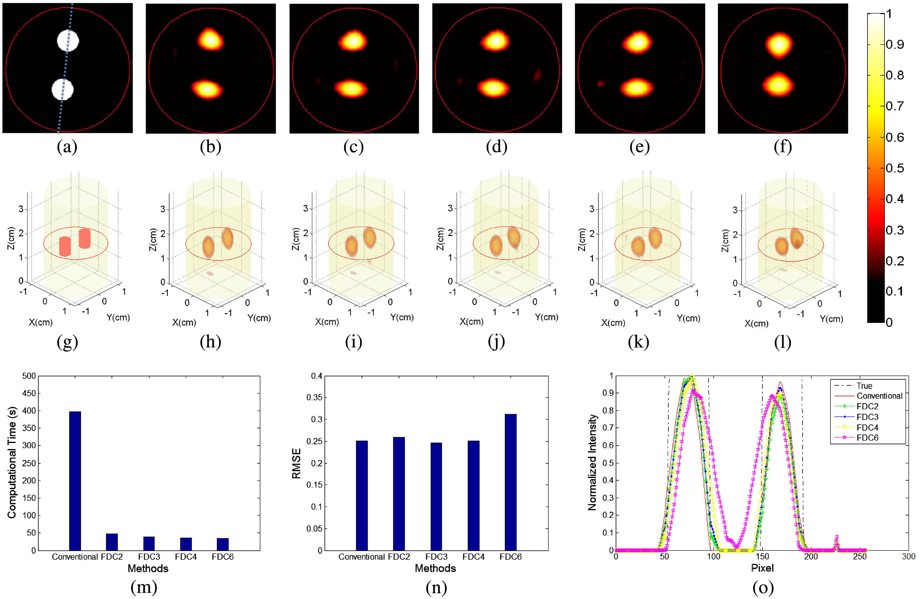
Figure 1 shows the results of the phantom experiment. Figures 1(a) and 1(g) are the slice and three-dimensional (3D) views of the true double targets. The corresponding reconstruction results obtained from the conventional method with the uncompressed original matrix equation are presented in Figs. 1(b) and 1(h). Figures 1(c)–1(f) are the slice views of the reconstruction results obtained from the FDC with 2, 3, 4, and 6 adjacent projections in each group, respectively (i.e., $N = 2$ , 3, 4, and 6), and Figs. 1(i)–1(l) are the corresponding 3D view of results. It can be seen that the reconstruction results obtained from the FDC are visually close to those obtained from the conventional method, except for the results from the FDC with 6 adjacent projections in each group (Figs. 1(f) and 1(l)). The locations of the two reconstructed fluorescence targets in Figs. 1(f) and 1(l) are not very accurate, because inadequate information is retained after the original fluorescence data is compressed excessively. The computational time by the FDC with 3 adjacent projections as shown in Fig. 1(m) is reduced to about 1/10th of the conventional method. The comparison of root-mean-square error (RMSE) and normalized intensity profiles along the dotted line in Fig. 1(a) is described in Figs. 1(n) and 1(o). The RMSEs [see Fig. 1(n)] and the profiles [see Fig. 1(o)] do not change much, except for the FDC with 6 adjacent projections in each group.

Figure 1.The results of the phantom experiment. (a) Slice and (g) 3D view of the true double fluorescence targets. (b) Slice and (h) 3D view of the reconstructed images obtained from the conventional method without data compression. (c)–(f) Slice and (i)–(l) 3D view of the reconstructed images obtained from the FDC strategy with 2, 3, 4, and 6 adjacent projections in each group. (m) Computational time consumed using different methods. (n) RMSEs and (o) normalized intensity profiles along the dotted line in (a) using different methods. All images are normalized by the maximal values of the results.

Figure 2 shows the results of the in vivo experiment. Figure 2(a) is the slice view of the CT image of the mouse at $z = 1.38 cm$ . The corresponding reconstruction results obtained from the conventional method are presented in Figs. 2(b) and 2(f). Figures 2(c)–2(e) are the slice views of the reconstruction results obtained from the FDC with 2, 3, and 6 adjacent projections in each group, respectively (i.e., $N = 2$ , 3 and 6), and Figs. 2(h)–2(j) are the corresponding 3D views of results. The reconstruction results obtained from the FDC [see Figs. 2(c)–2(e) and 2(g)–2(i)] are all visually close to the results obtained from the conventional method [see Figs. 2(b) and 2(f)], but the computational time by the FDC with 3 adjacent projections is reduced to about 1/10th of that needed to perform the conventional method [see Fig. 2(j)]. As shown in Figs. 2(k) and 2(l), the RMSEs and normalized intensity profiles along the dotted line in Fig. 2(a) are similar.

Figure 2.Results of the in vivo mouse experiment. (a) Slice view of the in vivo mouse. (b) Slice and (f) 3D view of the reconstructed images obtained from the conventional method. (c)–(e) Slice and (g)–(i) 3D view of the reconstructed images obtained from the FDC with 2, 3, and 6 adjacent projections. (j) Computational time consumed using different methods. (k) RMSEs and (l) normalized intensity profiles along the dotted line in (a) using different methods. All images are normalized by the maximal values of the results.

The results obtained using the FDC with 6 adjacent projections in the phantom experiment [see Figs. 1(f) and 1(l)] are not very accurate, but the results obtained using the FDC with 6 adjacent projections in the in vivo experiment [see Figs. 2(e) and 2(i)] are acceptable. The reason is that double fluorescence targets are included in the phantom experiment, and more information should be retained to maintain the reconstruction accuracy. So the number of adjacent projections in the FDC should have been less than 6 in the phantom experiment. Besides, the peaks of the normalized intensity profiles in the in vivo experiment [see Fig. 2(l)] obtained by the FDC did not match the true profile. This was caused by the fact that the locations of the reconstruction results deviate from the true location to some extent. The reconstruction accuracy may be improved by using anatomic a prior information from CT images in the process of reconstruction^[15], which will be studied in our future work.

In conclusion, a FDC strategy is proposed to accelerate the FMT reconstruction in this Letter. The strategy considers both the intra- and inter-projections’ redundant information, which can be reduced by the compression of fluorescence data. Then, the dimension of the FMT inverse problem is greatly reduced. This strategy is easy to implement because it does not need any additional analysis except for PCA. The reconstruction results of the phantom and in vivo experiments show that the proposed method can significantly increase the reconstruction efficiency while not significantly reducing the reconstruction accuracy compared with the conventional method without data compression.

References

[1] T. Wu, Y. Liu. Chin. Opt. Lett., 11, 021702(2013).

[2] M. Jia, S. Cui, X. Chen, M. Liu, X. Zhou, H. Zhao, F. Gao. Chin. Opt. Lett., 12, 031702(2014).

[3] V. Ntziachristos. Annu. Rev. Biomed. Eng., 8, 1(2006).

[4] W. Zou, J. Wang, D. D. Feng. J. Opt. Soc. Am. A., 30, 1464(2013).

[5] T. Correia, T. Rudge, M. Koch, V. Ntziachristos, S. Arridge. J. Biomed. Opt., 18, 086008(2013).

[6] X. Cao, X. Wang, B. Zhang, F. Liu, J. Luo, J. Bai. Biomed. Opt. Express., 4, 1(2013).

[7] P. Mohajerani, V. Ntziachristos. Opt. Lett., 38, 2324(2013).

[8] Y. Chen, X. Ma, X. Wang, S. Wang. Chin. Opt. Lett., 12, s21701(2014).

[9] R. C. Haskell, L. O. Svaasand, T. T. Tsay, T. C. Feng, M. S. McAdams, B. J. Tromberg. J. Opt. Soc. Am. A., 11, 2727(1994).

[10] S. R. Arridge. Inverse Probl., 15, R41(1999).

[11] J. Ripoll, M. N. Vesperinas, R. Weissleder, V. Ntziachristos. Opt. Lett., 27, 527(2002).

[12] D. A. Jackson. Ecology., 74, 2204(1993).

[13] D. Calvetti, S. Morigi, L. Reichel, F. Sgallari. J. Comput. Appl. Math., 123, 423(2000).

[14] F. Liu, X. Wang, D. Wang, B. Zhang, J. Bai. Ann. Biomed. Eng., 38, 3440(2010).

[15] X. Guo, X. Liu, X. Wang, F. Tian, F. Liu, B. Zhang, G. Hu, J. Bai. IEEE. Trans. Biomed. Eng., 57, 2876(2010).