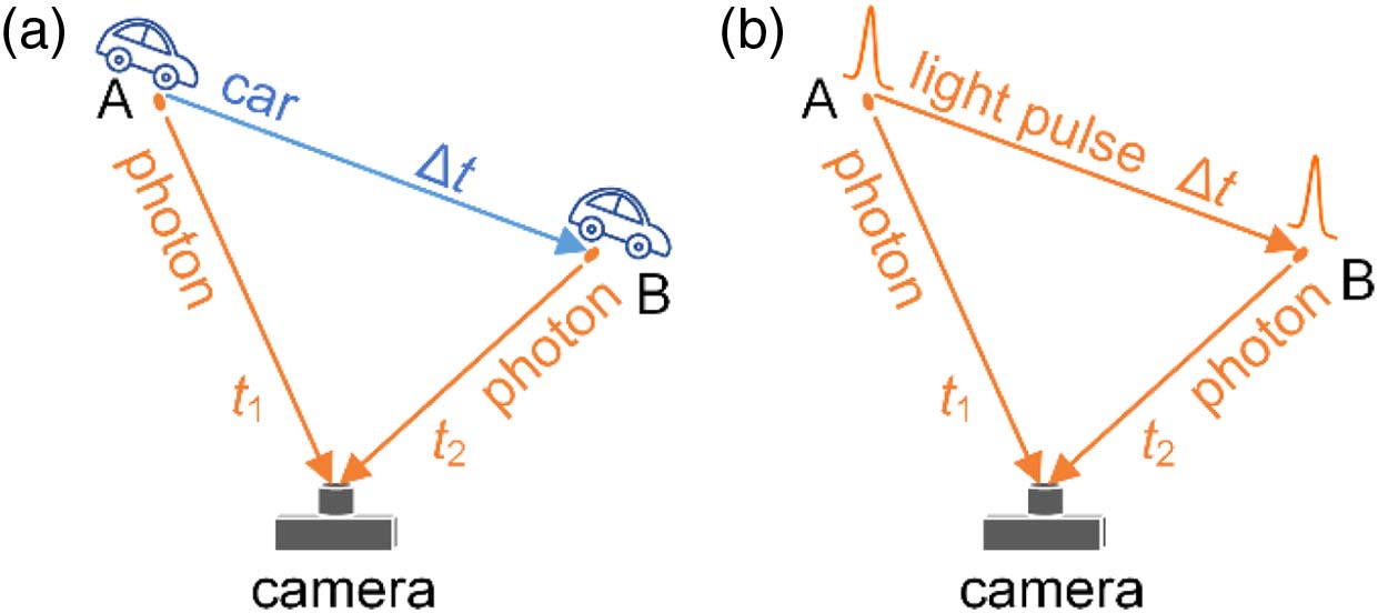
Fig. 1. Schematics of difference between imaging (a) a moving car and (b) a flying light pulse. Δt stands for the time during which the object moves from position A to position B, and t1 and t2 denote the time of flight for the scattered photons to propagate to the camera from positions A and B, respectively.

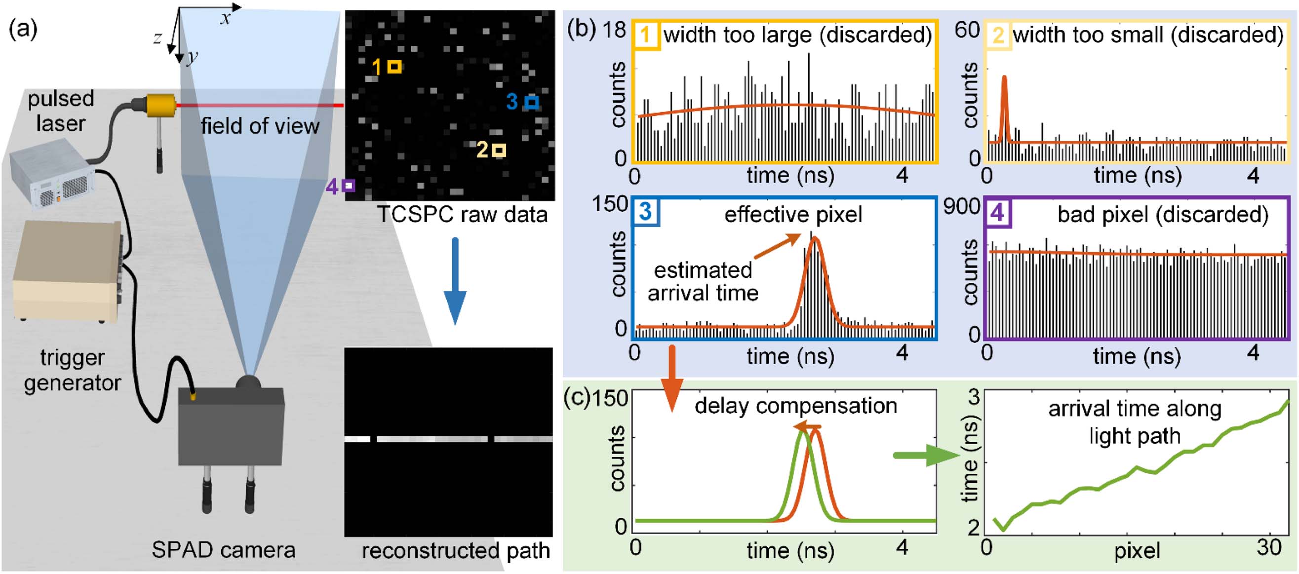
Fig. 2. Experimental system for light-in-flight measurement and data processing. (a) In the experiment, the pulsed laser and the SPAD camera are synchronized via a trigger generator. Placed at z=0  mm, a 636 nm pulsed laser emits pulses across the field of view of the SPAD camera. The SPAD camera, with a lens of 3.5 mm focal length, is located at z=535  mm. The object focal plane of the camera is the x–y plane at z=0  mm, having a field of view of 245  mm×245  mm. The SPAD camera collects the scattered photons from the propagating laser pulses and records a histogram at each pixel using TCSPC mode. (b) The raw data of the histograms is fitted with a Gaussian distribution. Histograms with widths too large or too small are discarded (pixels 1 and 2). Malfunctioning pixels with abnormally large counts are also discarded (pixel 4), leaving only effective pixels (pixel 3). (c) The arrival time of the scattered photons ta in the effective pixels is determined as the peak position of the fitted Gaussian distribution, and a pixel versus arrival time can be obtained. Consequently, the projection of the light path on the x–y plane, as well as the arrival times along the path is obtained, forming the (x, y, ta) three-dimensional data of light-in-flight.

Fig. 3. Optical model for the computation of propagation time t. α and θ are the angles of ∠CBG and ∠BAF, respectively. s and l are the lengths of BA and BE, respectively. BE is the projection of BD on the reference plane (RP).

Fig. 4. Reconstruction procedure for consecutive light paths. (a) For light path 1 (LP1), the reference plane (RP1) is the x–y plane containing the starting point 1 (S1). The spatial location of the projection (PP1), propagation angle, and ending point (E1) of LP1 are determined using the proposed geometric model. (b) E1 is used as S2 for the reconstruction of LP2, and RP2 is the x–y plane containing S2. The equation of LP2 and the position of E2 can be obtained. (c) In the same manner, LP3 and E3 are determined with RP3.

Fig. 5. Experimental results of the propagation angle estimation. (a) Angle error resulting from using different numbers of tai for the estimation of α. (b) Calculated propagation time t with respect to arrival time ta at different propagation angles. (c) The variation of measured full width at half maximum for a laser pulse with respect to its propagation angle α, caused by the relativistic effects.

Fig. 6. Experimental 4D reconstruction of light-in-flight. (a) A reconstruction of a laser pulse reflected by two mirrors is demonstrated. The RMSEs of the reconstruction (red line) to the ground truth (dashed line) in position and time are 1.75 mm and 3.84 ps, respectively. (b) The difference between the calculated propagation time t (red line) and measured arrival time ta (blue line) at each recorded frame. The propagation time is in good agreement with the ground truth (dashed line), demonstrating a feasible compensation for the relativistic effects via the proposed scheme.