
J. B. Ohland, U. Eisenbarth, B. Zielbauer, Y. Zobus, D. Posor, J. Hornung, D. Reemts, V. Bagnoud, "Ultra-compact post-compressor on-shot wavefront measurement for beam correction at PHELIX," High Power Laser Sci. Eng. 10, 03000e18 (2022)
- High Power Laser Science and Engineering
- Vol. 10, Issue 3, 03000e18 (2022)
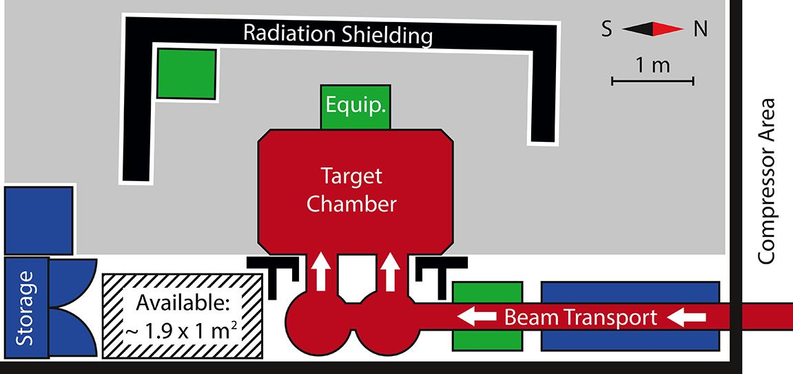
Fig. 1. Scale sketch of the PHELIX target area before the installation of the PTAS. The DM will be placed in the compressor area to the right, while the available space for the PTAS is indicated by the ruled area on the left. The light gray region indicates the area reserved for user equipment and personnel access.
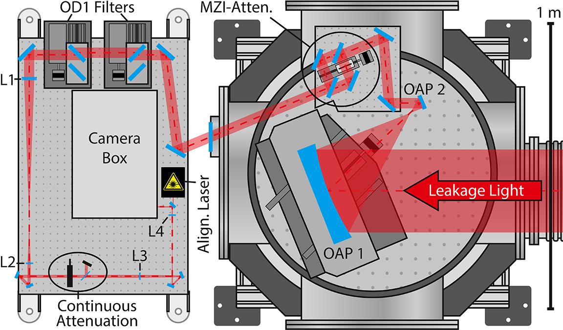
Fig. 2. Scale schematic of the PTAS. The intermediate focal diagnostic is not shown for clarity. The other main components are labeled (‘L’ for lenses) and described in the text.
Fig. 3. The NF (left) and absolute, uncorrected WF (right) at the PTAS, recorded on-shot using the largest possible aperture.
Fig. 4. An etched tungsten needle is used to mark the position of the focal spot (center). A bit of dust has stuck on its tip. The large caustics are created by backlighting, which is used in order to see the shadow of the needle.
Fig. 5. Scale schematic of the intermediate focal diagnostic in side view (left) and top view (right), observing the backwards propagating alignment beam. The needle and the diagnostic mirrors can be moved in and out of the beam, while the microscope can be moved in three axes in order to change the viewing position. The other possible states of the diagnostic are drawn as transparent overlays.
Fig. 6. Schematic of the CLAWS concept.
Fig. 7. Sketch of the target chamber area, indicating a possible configuration during the calibration routine.
Fig. 8. The unoptimized (left) and optimized (right) focal spots of a copper OAP at the target position, recorded with a 16-bit CMOS camera, installed in CLAWS. The intensity is estimated for a 100 J, 500 fs pulse.
Fig. 9. The encircled energy over the radius from the point of largest intensity, taken for the focuses shown in Figure 8 .
Fig. 10. The unoptimized (left) and optimized (right) WFs corresponding to the focuses shown in Figure 8 , recorded using CLAWS. The WFs are measured relative to the reference generated using the pinhole. The unoptimized WF features an RMS of 0.202 , while it is reduced to 0.052
 after optimization.
, while it is reduced to 0.052 after optimization. Fig. 11. A sketch of the PHELIX compressor, including the gratings, the DM and the directions to the compressor beam sensor (‘COS’) and the PTAS.
Fig. 12. A qualitative comparison between FFs (a) measured at the compressor exit and (b) measured at the PTAS at the same time. No beam correction was applied.
Fig. 13. Transparency of the polystyrene foil targets, plotted over their thickness. The estimated intensities are color coded, while different shot configurations are indicated by the shape of the data points. The data set displayed as triangles was taken from a previous beam time (P155).


Set citation alerts for the article
Please enter your email address

© Copyright 2018-2021 | Chinese Laser Press. All Rights Reserved 沪ICP备15018463号-20