Microwave heating is widely used in food health care, wood processing, ceramic sintering^[1] and other fields. It makes polar molecules in the heated medium interact rapidly in a short time through electromagnetic field to generate a large amount of heat, thus it has the advantages of fast heating rate, green environmental protection, etc. However, it also has the uneven temperature heating and local overheating caused by the simultaneous existence of hot spots and cold spots^[2]. Due to the huge power required by industrial microwave heating equipment, one microwave source can not meet the requirements, hence there are usually multiple microwave sources working together.

Chan T et al^[3] analyzed that the symmetrical distribution of feed ports can improve the coupling degree of feed ports by microwave heating model of four feed ports. Kusturee Jeni et al^[4] and Wang Shunmin et al^[5] proposed that the microwave heating equipment with multiple feed ports could make the internal temperature of microwave oven more uniform. Zhou Mingchang^[6] used COMSOL to simulate a cylindrical microwave resonator with ten feed ports. The results show that the increase of the number of feed ports can greatly improve the uniformity of dielectric heating. However, nonuniformity of microwave heating still exists. Dai Chengjun^[7] analyzed the heat energy change in the microwave heating device, and obtained the unsteady differential equation and the first-order inertial transfer function with delay by Laplace transform simulation, which simulated the real-time process of coal microwave heating. Yang Biao et al^[8] proposed a numerical calculation model for microwave heating of moving materials by distribution relationship between voltage and current on the transmission line, which could effectively suppress the sudden change of microwave heating temperature. Based on the microwave heating mechanism model, Zhong Jiaqi et al^[9] verified the effectiveness of its temperature tracking control strategy by microwave heating short waveguide model.

Because of the non-uniformity of microwave heating and the unknown loss of actual circuit, this paper chooses water with good quality and low price as the heated medium. First, the power of magnetron is roughly determined by differential static modeling, which is used for COMSOL simulation and calculation of heat source in MATLAB simulation. Microwave non-uniform heating, that is, the distribution of heat source, can be reasonably assumed according to the electric field distribution in water medium in COMSOL simulation. Moreover, the temperature distribution simulated by MATLAB is roughly consistent with that simulated by COMSOL, which verifies the effectiveness of the model. Assuming that the temperature in the heated medium can be obtained by MATLAB simulation, the temperature in the edge of the water medium decreases, and the temperature in the center part is about T, so the temperature T can be regarded as its steady state. That is, after stopping heating, the temperature in all parts of the water medium tends to be neutral, and the microwaves that have not yet reacted with water also react with water at this time, and the temperature at all points in the water reaches the same after a period of time. According to the COMSOL simulation of uneven microwave heating point temperature, some representative points near the temperature T are found, and the actual temperature changes of these points in the heating process are compared to find out the best point as the control object. After that, the point that can best reflect the temperature change trend in the microwave heating device and any other points in the medium are controlled by expert PID, which verifies the advantages of taking the temperature rise equilibrium point as the research object for microwave controlled heating.

The microwave heating system consists of an electromagnetic wave generator and a metal microwave resonant cavity which can reflect microwave to the surface of the heated object. Microwave resonator is a space geometry composed of a cylinder with a height of 0.8 m and a bottom diameter of 0.8 m; The contact area between the internal stainless steel bracket and the inner wall of the microwave oven is $ 4 \times 0.23\;{\text{m}} \times 0.23\;{\text{m}} $. Microwave heating uses its affinity with polar molecules to heat, that is, microwave energy passes through insulating materials without consuming energy, and is absorbed when encountering polar molecules—water, thus achieving the effect of microwave heating. Tap water is used as the heated medium. The heat dissipation link is mainly divided into four parts from inside to outside: tap water, ceramic cup, air and microwave oven wall. According to different heat transfer mechanisms, it can be divided into three basic modes: heat transfer, heat convection and heat radiation. One-dimensional calculation is made in any direction with the side of the cylinder as the bottom. There are five magnetrons with rated power of 1 kW on the periphery of microwave oven cavity, which transmit the energy generated by them into the oven to heat the medium through five rectangular waveguides. All the five magnetrons have only two states: on and off. The microwave resonant cavity is shown in Fig.1.

In actual industrial production, the way of heat transfer does not exist alone, but has a combination of various ways of heat transfer. The compound heat transfer process of microwave oven is divided into three parts:

(1) The outer wall of the ceramic cup transfers heat to the inner surface of microwave oven through natural convection and heat radiation in limited space.

(2) The inner surface of microwave oven diffuses heat to the outer surface of microwave oven by heat conduction.

(3) Heat diffuses into the air by heat convection on the outer surface of microwave oven.

One-dimensional schematic diagram of heat loss of microwave oven equipment during operation is shown in Fig.2.

According to the Fourier Law, the Newton’s cooling formula^[10] and Stefan-Boltzmann Law, the heat loss $ {Q_{{\mathrm{San}}\_k}} $ of microwave heating system is obtained by the difference method at time k:

$ {Q_{{\mathrm{San}}\_k}} = {\left( {\dfrac{1}{{\left( {{h_1} + {h_2}} \right)}} + \dfrac{\delta }{\lambda } + \dfrac{1}{{{h_3}}}} \right)^{ - 1}} \cdot \left( {{T_k} - {T_{k - 1}}} \right) \cdot A{\text{ = }}K \cdot \left( {{T_k} - {T_{k - 1}}} \right) \cdot A $ (1)

In Eq. (1), $ {h_1} $ and $ {h_2} $ are the natural commutation coefficient and radiation heat transfer coefficient in limited space; $ \delta $ is the thickness of the outer wall of microwave oven (mainly composed of stainless steel); $ \lambda $ is the heat transfer coefficient of the outer wall of microwave oven; $ {h_3} $ is the convective heat transfer coefficient of general gas; $ {T_k} $ and $ {T_{k - 1}} $ are the temperature of water medium and outside air (the room temperature) at time k, respectively; A is the stainless steel wall area of microwave oven; K is the total heat transfer coefficient.

The difference model of medium temperature at any time when microwave oven works is:

$ {T_k} = {T_{k - 1}} + \dfrac{{{Q_k} - {Q_{{\mathrm{San}}\_k - 1}}}}{{{{{c}}_1}{m_1} + {{{c}}_2}{m_2}}} $ (2)

Where $ {Q_k} $ is the microwave input power at time k, and a control quantity u can be added here to control the opening and breaking of the magnetron; $ {c_1} $ and $ {c_2} $ are the specific heat capacity of water and ceramic cup respectively, $ {m_1} $ and $ {m_2} $ are the mass of water and ceramic cup respectively. The water medium and ceramic cup are approximately regarded as a whole to simplify the model.

Because the purity of stainless steel on the outer wall of microwave oven is unknown in the actual equipment environment, the actual heat transfer coefficient K and magnetron power $ {Q_k} $ cannot correspond to the theoretical value due to the aging of magnetron and the influence of actual circuit. 4 kg, 5 kg and 6 kg of tap water are used for heating, and a temperature measuring point in the middle of the medium is taken for measurement. The cooling process corresponds to Eq. (2), and the actual K value is 2.05, which can better reflect the temperature drop process; When the actual power $ {Q_k} $ of magnetron is 3830 W, which is obtained by taking the temperature rise process corresponding to Eq. (2), it is more in line with the actual situation. Different water mass makes the temperature delay different. The temperature rise delay of 4 kg, 5 kg and 6 kg tap water is the closest to the actual temperature rise process by taking 90 s, 100 s and 110 s respectively. Water quality (${m_1}$) and heating delay ($ {k_{{\mathrm{delay}}}} $) roughly satisty the following equatopn:

$ {k_{{\mathrm{delay}}}} = 10{m_1} + 50 $ (3)

Randomly take 5.4 kg of water medium for the Bang-Bang control heating at a set temperature of 70 ℃. The practical results obtained by the Bang-Bang control heating, the theoretical results obtained by MATLAB based on the difference model (Eq. (2)) of medium temperature, are all shown in Fig.3. Fig.3 shows that the static difference model is consistent with the actual heating and cooling process, and the actual input power $ {Q_k} $ is about 3830 W, which can be used to calculate the heat source input of MATLAB dynamic model and COMSOL simulation model. The Bang-Bang control strategy is:

$ P\left( k \right) = \left\{ \begin{gathered} {Q_k},\quad {T_k} \lt {T_{sk}} \\ 0,\;\;\quad {T_k} \geqslant {T_{sk}} \\ \end{gathered} \right. $ (4)

In Eq. (4), $T_{sk}$ is the set temperature, which is adjust able, and $ {T_k} $ is the actual temperature of water medium at time k；$ P\left( k \right) $ is the actual power of microwave input at time k.

To observe the temperature at any time and at any position in the microwave oven and understand the heating situation, the finite difference method is used to simplify the model (the thermal convection and radiation of the air in the device are ignored). Because the experimental device is a cylinder, it matches the three dimensions of the device and has an internal heat source. Taking the element control body($ {\mathrm{d}}V = r \cdot {\mathrm{d}}\varphi \cdot {\mathrm{d}}r \cdot {\mathrm{d}}{\textit{z}} $) in the cylindrical coordinate system, the energy conservation relationship is established. The general form of the unsteady heat conduction differential equation is (the thermal conductivity is treated as a constant) ^[11]:

$ \rho c\dfrac{\partial T}{\partial t}=\lambda\Bigg(\dfrac{1}{r}\dfrac{\partial T}{\partial r}+\dfrac{\partial^2T}{\partial r^2}+\dfrac{1}{r^2}\dfrac{\partial^2T}{\partial\varphi^2}+\dfrac{\partial^2T}{\partial\text{z}^2}\Bigg)+\mathit{\Phi} $ (5)

In Eq. (5), $ \rho $ and c are density and specific heat capacity of the medium; $ \lambda $ is thermal conductivity of the medium; T is the actual temperature of the medium at time t; r is the distance between the selected element and the central axis of the cylinder; $ \varphi $ is the angle between the selected element and the x-axis direction; z is the height of the selected element; $ \mathit{\Phi} $ is the intensity of internal heat source.

Because of the circular symmetry, the 3D problem is simplified to a 2D problem:

$ \rho c\dfrac{\partial T}{\partial t}=\lambda\Bigg(\dfrac{1}{r}\dfrac{\partial T}{\partial r}+\dfrac{\partial^2T}{\partial r^2}+\dfrac{\partial^2T}{\partial\text{z}^2}\Bigg)+\mathit{\Phi} $ (6)

Taking the half section of a cylinder as the research object, different materials are partitioned, and the 2D schematic diagram is shown in Fig.4.

In Fig.4, W, G, A and B respectively represent different medium of water, ceramic, air and stainless steel, and the material parameter (density, specific heat capacity and thermal conductivity) values of each layer are shown in Table 1; their subscripts represent different areas meshed by use of finite difference method. The boundaries in the direction r are $ 0,{r_1},{r_2},{r_3},{r_4} $; boundaries in the z direction are $ 0,{{\textit{z}}_1},{{\textit{z}}_2}, $${{\textit{z}}_3}, {{\textit{z}}_4},{{\textit{z}}_5}, {{\textit{z}}_6},{{\textit{z}}_7} $.

The outside air temperature is $ {T}_{{\mathrm{s}}\_{\mathrm{right}}}={T}_{{\mathrm{s}}\_{\mathrm{up}}}={T}_{{\mathrm{s}}\_{\mathrm{down}}}=20 $ ℃; $ {h_{{\mathrm{s}}\_{\mathrm{right}}}} $, $ {h_{{\mathrm{s}}\_{\mathrm{up}}}} $ and $ {h_{{\mathrm{s}}\_{\mathrm{down}}}} $ are the air convective heat transfer coefficients to the right, above, and below the microwave resonant cavity in Fig.4. The convective heat transfer coefficient^[11] is $ {h_{{\mathrm{s}}\_{\mathrm{right}}}} = {h_{{\mathrm{s}}\_{\mathrm{up}}}} = {h_{{\mathrm{s}}\_{\mathrm{down}}}} = 10\;{\mathrm{W}}/\left( {{{\mathrm{m}}^2} \cdot {\mathrm{K}}} \right) $. The display difference format is used for difference. Differentiation of heat conduction differential equations and boundary conditions in all regions in Fig.4 is carried out to establish a dynamic model of temperature distribution in microwave oven resonant cavity:

① There is an internal heat source in the water medium (that is, the water medium absorbs microwave), so the differential heat conduction equation in $ {W_1} $ region is divided into:

$ \begin{split} & \rho_1c_1\dfrac{T\left(j,k,n+1\right)-T\left(j,k,n\right)}{\Delta\tau}=\lambda_1\Bigg(\dfrac{1}{r_j}\dfrac{T\left(j+1,k,n\right)-T\left(j,k,n\right)}{\Delta r}+ \\ & \quad\quad\dfrac{T\left(j+1,k,n\right)-2T\left(j,k,n\right)+T\left(j-1,k,n\right)}{\left(\Delta r\right)^2}+\dfrac{T\left(j,k+1,n\right)-2T\left(j,k,n\right)+T\left(j,k-1,n\right)}{\left(\Delta\text{z}\right)^2}\Bigg)+\mathit{\Phi}\end{split} $ (7)

Make ${e}_{1}=\dfrac{\Delta \tau {\lambda }_{1}}{{\rho }_{1}{c}_{1}}；{r}_{j}=j\cdot \Delta r；{{\textit{z}}}_{k}=k\cdot \Delta {\textit{z}}；{f}_{1}=\dfrac{\Delta \tau {\lambda }_{1}}{{\rho }_{1}{c}_{1}}\cdot \dfrac{1}{{\left(\Delta r\right)}^{2}}；{g}_{1}=\dfrac{\Delta \tau {\lambda }_{1}}{{\rho }_{1}{c}_{1}}\cdot \dfrac{1}{{\left(\Delta {\textit{z}}\right)}^{2}}$

$ \begin{split}T\left(j,k,n+1\right)= & \left(\dfrac{1}{j}+1\right)\cdot f_1\cdot T\left(j+1,k,n\right)-\left(\dfrac{1}{j}\cdot f_1+2f_1+2g_1-1\right)\cdot T\left(j,k,n\right)+ \\ & f_1\cdot T\left(j-1,k,n\right)+g_1\cdot\left(T\left(j,k-1,n\right)+T\left(j,k+1,n\right)\right)+\dfrac{e_1\mathit{\Phi}}{\lambda_1}\end{split} $ (8)

Where j is the number of grid nodes in the r direction; k is the number of grid nodes in the z direction; n is the number of time nodes; $ \Delta r $ is the step size in the r direction; $ \Delta {\textit{z}} $ is the step size in the z direction; $ \Delta \tau $ is the time step.

② The left boundary in the r direction of the area is adiabatic, and the right boundary is ceramic. Make $ a = 1,2,3,4 $; $ {p_a} = {{{\lambda _a}} \mathord{\left/ {\vphantom {{{\lambda _a}} {\Delta r}}} \right. } {\Delta r}} $; $ {\lambda _1},{\lambda _2},{\lambda _3},{\lambda _4} $ are the thermal conductivity coefficient of water medium, ceramic medium, air medium, and stainless steel medium.

$ \begin{split} & \dfrac{{\partial T\left( {1,k,n + 1} \right)}}{{\partial r}} = 0;\quad r = \Delta r \\ & {\lambda _1}\dfrac{{\partial T\left( {j,k,n + 1} \right)}}{{\partial r}} = {\lambda _2}\dfrac{{\partial T\left( {j + 1,k,n + 1} \right)}}{{\partial r}};\quad r = {r_1} \end{split} $ (9)

Differentiation and simplification are carried out to obtain:

$ \begin{split} &T\left( {1,k,n + 1} \right) = T\left( {2,k,n + 1} \right);\quad r = \Delta r \\ & T\left( {j + 1,k,n + 1} \right) = \dfrac{{{p_2}}}{{\left( {{p_1} + {p_2}} \right)}} \cdot T\left( {j + 2,k,n + 1} \right) + \dfrac{{{p_1}}}{{\left( {{p_1} + {p_2}} \right)}} \cdot T\left( {j,k,n + 1} \right);\quad r = {r_1} \end{split}$ (10)

In the z direction of water region, a difference equation is established to solve it.

According to steps ① and ②, difference equations are established and simplified according to different points in each region. The heat transfer between the stainless steel wall and the outside air is heat convection, and the boundary differential equation is slightly different. The rightmost boundary is:

$ - {\lambda _4}\dfrac{{\partial T\left( {j,k,n + 1} \right)}}{{\partial r}} = h\left( {T\left( {j + 1,k,n + 1} \right) - {T_{{\mathrm{s}}\_{\mathrm{right}}}}} \right)；r = {r_4} $ (11)

Make $ d = \dfrac{{{\lambda _4}}}{{h \cdot \Delta r}} $, differentiation was carried out:

$ T\left( {j + 1,k,n + 1} \right) = \dfrac{d}{{1 + d}} \cdot T\left( {j,k,n + 1} \right) + \dfrac{{{T_{{\mathrm{s}}\_{\mathrm{right}}}}}}{{1 + d}} $ (12)

The stability limits of internal node discrete equation and boundary node discrete equation are as follows^[11]:

$ F{o_\Delta } = \dfrac{{\lambda \cdot \Delta \tau }}{{\rho \cdot c \cdot {{\left( {\Delta r} \right)}^2}}} \leqslant 0.5；F{o_\Delta } \leqslant \dfrac{1}{{2\left( {1 + B{i_\Delta }} \right)}}；B{i_\Delta } = \dfrac{{h \cdot \Delta r}}{{{\lambda _4}}} $ (13)

Because the ceramic cup wall and stainless steel wall are only about 5mm, 2.5mm is the most suitable for $ \Delta r $. The radius r direction and z direction have the same restrictions, so in order to simplify the model, make $ \Delta r = \Delta {\textit{z}} = 2.5\;{\rm{mm}} $. $ \Delta \tau \leqslant 0.129\;7\;{\rm{s}} $ is obtained from Eq. (13), so make $\Delta \tau = 0.1\;{\rm{s}}$.

Set the mass of water to 5 kg, since the ceramic cup is a cylindrical container with a radius of 0.08 m and a height of 0.33 m. the height of the water medium is 0.24 m, the volume $ {V_{{\mathrm{water}}}} $ of the water medium in the ceramic cup can be obtained . the intensity of internal heat source is:

$ \mathit{\Phi}=\dfrac{Q_k}{V\mathrm{_{\mathit{\mathrm{water}}}}}=\dfrac{3\; 830}{3.14\times\left(0.08\right)^2\times0.24}\approx794\; 105\left(\mathrm{W}/\mathrm{m}^3\right) $ (14)

In COMSOL, the space geometric model is designed according to the size and material of the actual device, and the 1/2 full-size model (Fig.5) is taken, that is, three feed ports are fed with $ {{{Q_k}} \mathord{\left/ {\vphantom {{{Q_k}} 2}} \right. } 2} $ microwave, and temperature (℃) distribution at heating for 465 s, the heating step is 1 s (Fig.6). The electric field distribution in r direction and z direction at the center of water medium is shown in Fig.7.

In Fig.7, L is the distance from origin O in r and z directions. As can be seen from Fig.7, the electric field in z direction decreases rapidly from the edge of water medium (the two blue points represent the upper edge position and the lower edge position of the water medium respectively) to 40 mm inside, and the middle part tends to be roughly stable. The electric field in r direction is always in a weak state.

To correspond with the coordinates in MATLAB simulation, the coordinates in the following text are expressed in the form of (x/mm, y/mm, z/mm). In MATLAB, the internal heat source distribution is adjusted according to the electric field intensity, and the simulation time is 465 s and the heating step is 0.1 s. Taking the three-bit section between the point (0, 0, 520) and the point (0, 395, 520) in the r direction, and taking the three-bit section between the point (0, 65, 0) and the point (0, 65, 795) in the z direction (based on Fig.5), when simulating 465 s, the temperature pairs of each 3D section point are shown in Fig.8.

The main reason the water medium simulation exceeds 100 ℃ in Fig.8 is highlighting the inhomogeneity of microwave heating, thus the temperature is not limited in simulation. Due to the complexity of the electromagnetic field distribution inside the microwave resonant cavity, MATLAB simulation cannot truly simulate irregular electromagnetic fields. Therefore, the simulation results of MATLAB and COMSOL are relatively similar in the r direction and slightly different in the z direction, but the overall trends are similar, which verifies the correctness of the finite difference model.

After stopping heating, because the water medium is liquid, the uneven temperatures will eventually neutralize each other, so that the temperature of the water medium will eventually tends to T. It can be assumed that the heat source is uniformly distributed in the water medium in MATLAB simulation, and the MATLAB temperature distribution is shown in Fig.9(a). The temperature distribution of MATLAB when the heat source is unevenly distributed is introduced in Fig.9(b).

As can be seen from Figure 9, assuming uniform microwave heating, the temperature distribution of water medium is uniformly T, and the temperature at the boundary is slightly lower than that at the central part. At this point, the coordinates of the three-dimensional cutoff points similar to temperature T can be found in the simulation results of uneven heating in MATLAB and COMSOL, such as A (20, 0, 475) and B (20, 0, 455). These 3D intersections are called the equilibrium points of temperature rise in the heating process of water medium, which can reflect the temperature change trend of the whole water medium in the microwave heating process to the greatest extent.

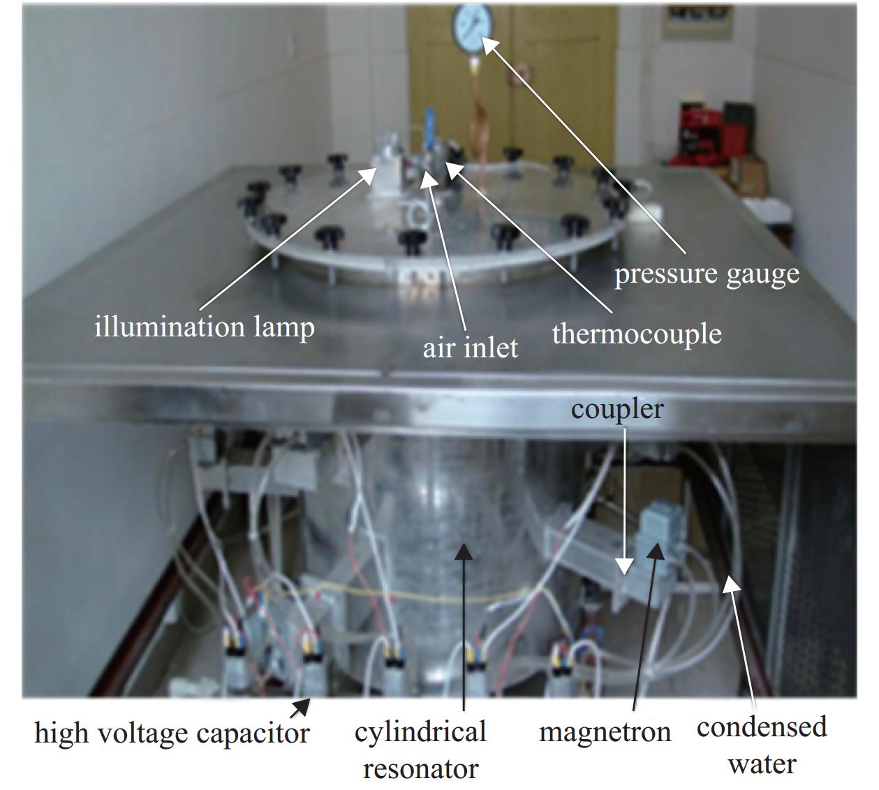
To better demonstrate the particularity of temperature rise balance point in control, a microwave heating experimental device was set up for experimental verification. In the experimental equipment, three-phase AC power supply provides input voltage for the normal operation of high voltage transformer (GAL-800E-4). The output end of the high-voltage transformer outputs about 4 V and 2000 V AC voltages, in which 4 V AC supplies power to the filament of the magnetron. The output end of 2000 V AC and 1$ {\text{μ}}\text{F} $ capacitor form a half-wave rectifier circuit to output 4000 V DC negative high voltage to supply power to the cathode of the magnetron. The anode of the magnetron is grounded^[12], which forms a closed loop. 24V DC power supply (LM35-22B24) provides power for PLC (Programmable Logic Controller). PLC obtains the digital signal converted by K-type thermocouple and analog module (EM231) to obtain the current temperature to provide control signal. It can change the working state of magnetron by controlling the on-off of AC relay coil through ladder diagram, and play the role of isolating AC and DC. The diagram of microwave heating control system is shown in Fig.10.

In a real microwave heating experiment, the peripheral point C (40, 0, 520), the central point D (0, 0,420) and the temperature rise equilibrium points A and B in the water medium were selected as the research objects, and K-type thermocouples of the same model were placed near these four points. When 5 kg tap water was heated to the set temperature of 70 ℃, the magnetron was disconnected and the temperature change trend at different points during this process was observed, as shown in Fig.11.

As can be seen from Fig.11, the temperature of water medium varies from place to place due to the inhomogeneity of microwave heating. After the heating process of about 465 s, the water medium absorbs the residual microwave, and the neutralization of water temperature is dominant. At about 675 s, the overall temperature in all parts of the water medium is about 83.5 ℃, and then the heat dissipation occupies a dominant position. Point C is located in the periphery of water medium, absorbing more microwave energy and heating up quickly. Point D, which is in the center of water medium, absorbs less microwave, and mainly depends on the neutralization reaction of water to heat up after stopping heating. There is still a small amount of overshoot when heating is stopped at point A, which is roughly stable at about 83.5 ℃ compared with when heating is stopped at Point B. The temperature rise equilibrium point B is selected as the control object in the follow-up experiment, which can best reflect the overall uniform temperature of the heated liquid medium at each time.

In three microwave heating experiments, temperature rise equilibrium point B, peripheral point C and central point D are taken as control objects, and incremental expert PID is used to control them. The control rules are shown in Table 2, in which u represents the control quantity output by the controller, and the temperature change trend of each point is shown in Fig.12.

It can be seen from Fig.12 that the overshoot at peripheral point C is about 1.4 ℃, and the time to reach the set temperature is about 260 s. The B-ultrasound adjustment of temperature rise equilibrium point is about 1.9 ℃, and the time to reach the set temperature is about 400 s. The D overshoot at the center point is about 3.7 ℃, and the time to reach the set temperature is about 500 s. According to the analysis of microwave input power and water medium quality, when the temperature at point C reaches the designated temperature of 70 ℃, temperatures at other locations within the water medium have not yet attained the preset temperature. Likewise, when the temperature at point D reaches the designated temperature, the peripheral regions of the water medium have already exceeded the preset temperature. Consequently, the desired control outcome cannot be achieved in either case. However, when the temperature at the equilibrium point of temperature rise, denoted as point B, reaches the preset temperature, the phenomenon of liquid diffusion ensures that temperatures at other points within the water medium closely approximate the set temperature of 70 ℃. Therefore, designating the temperature rise equilibrium point B as the heating target offers the most effective means of reflecting the overall temperature trend of the heated liquid medium. Furthermore, when the controller engages in its control operation, the magnetron switching frequency is moderate, contributing to an extended operational lifespan of the magnetron, compared to frequent switching.

Due to the inherent non-uniformity of microwave heating, the approach of haphazardly positioning temperature sensors for the measurement of the heated medium's temperature is deemed imprudent. Hence, this paper introduces a dynamic finite difference model as a methodology to identify temperature rise equilibrium points. Multiple such points are identified and subsequently tested to discern the most optimal equilibrium point for microwave heating control. The principal research focus of this paper can be segmented into three primary components:

(1) According to the physical structure of the microwave heating device, the static differential modeling is carried out to obtain the actual power of the magnetron in full operation, which provides data support for the later simulation.

(2) The temperature distribution of multi-media in 3D space is modeled, and the distribution of microwave heat source is obtained by simulating the distribution of electric field in water medium in COMSOL. The accuracy of the 3D finite difference model is verified by comparing MATLAB with COMSOL simulation of microwave heating. After that, assuming that the uniform temperature of water medium is obtained by 3D finite difference model when microwave heating is uniform (microwave heat source is uniformly distributed), the 3D cross-section points close to the temperature in COMSOL simulation model are found out, and these temperature equilibrium points can reflect the whole temperature change trend of medium in microwave heating device to the greatest extent.

(3) Subsequently, through a series of straightforward microwave heating experiments, the equilibrium point of temperature rise exhibiting the most favorable performance characteristics is selected for microwave heating control. In conclusion, this selected point, when employed as the control object, is subjected to intelligent control alongside other control objects to validate its superiority in the context of microwave heating control.

The experimental results show that the microwave heating control method based on the dynamic finite difference method can transform the non-uniformity problem of microwave heating into the problem of finding the best place to replace the uniform heating point of the whole medium, and then it can be solved visually by MATLAB and COMSOL. This method has a good application prospect for the medium with good thermal conductivity (especially liquid medium) in the actual industrial production of microwave heating.

References

[3] Chan T V C T, Reader H C. Computational design of a multiplex magron cavity[C]Proceedings of IEEE AFRICON’96. 1996: 523527.
[6] Zhou Mingchang. Study on numerical simulation of microwave heating temperature control[D]. Mianyang: Southwest University of Science Technology, 2020.
[7] Dai Chengjun. The design development of the microwave activation equipment on the industry[D]. Mianyang: Southwest University of Science Technology, 2012.
[8] Yang Biao, Wang Shili, Guo Linjia, et al. Numerical calculation of temperature uniformity in microwave heating based on moving mesh[J]. Control and Decision, 34, 113-120(2019).
[9] Zhong Jiaqi, Liang Shan, Xiong Qingyu.
[10] Zheng Hongfei. Fundamentals of thermodynamics heat transfer[M]. Beijing: Science Press, 2016.
[11] Liu Yanfeng, Liang Xiujun, Gao Zhengyang, et al. Heat transfer[M]. Beijing: China Electric Power Press, 2021.
[12] Zhou Mingchang, Li Shaofu. Multi-feed microwave heating temperature control system based on numerical simulation[J]. Journal of Microwaves, 35, 92-96(2019).
Set citation alerts for the article
Please enter your email address
© Copyright 2018-2021 | Chinese Laser Press. All Rights Reserved 沪ICP备15018463号-20