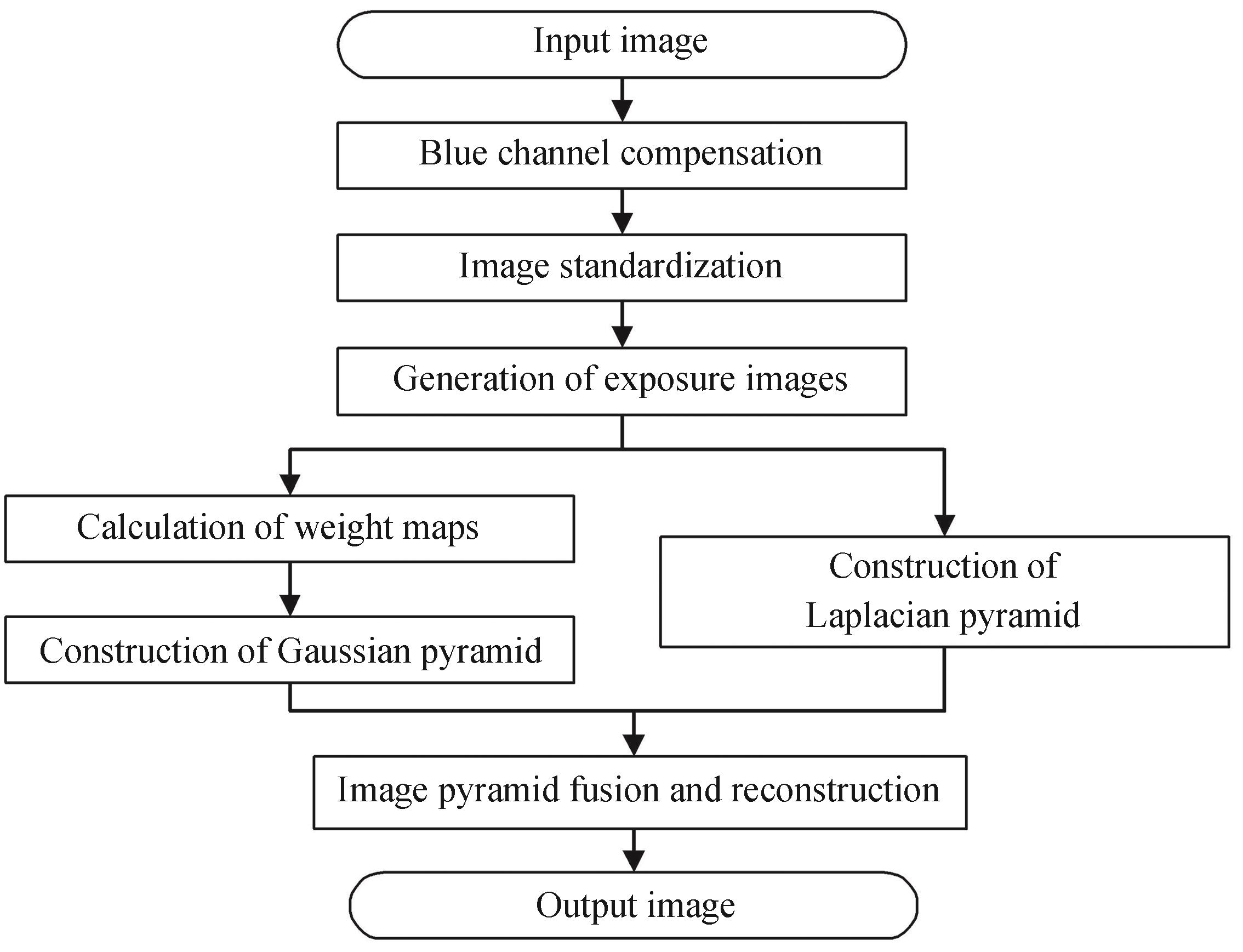
Fig. 1. Algorithm flow chart
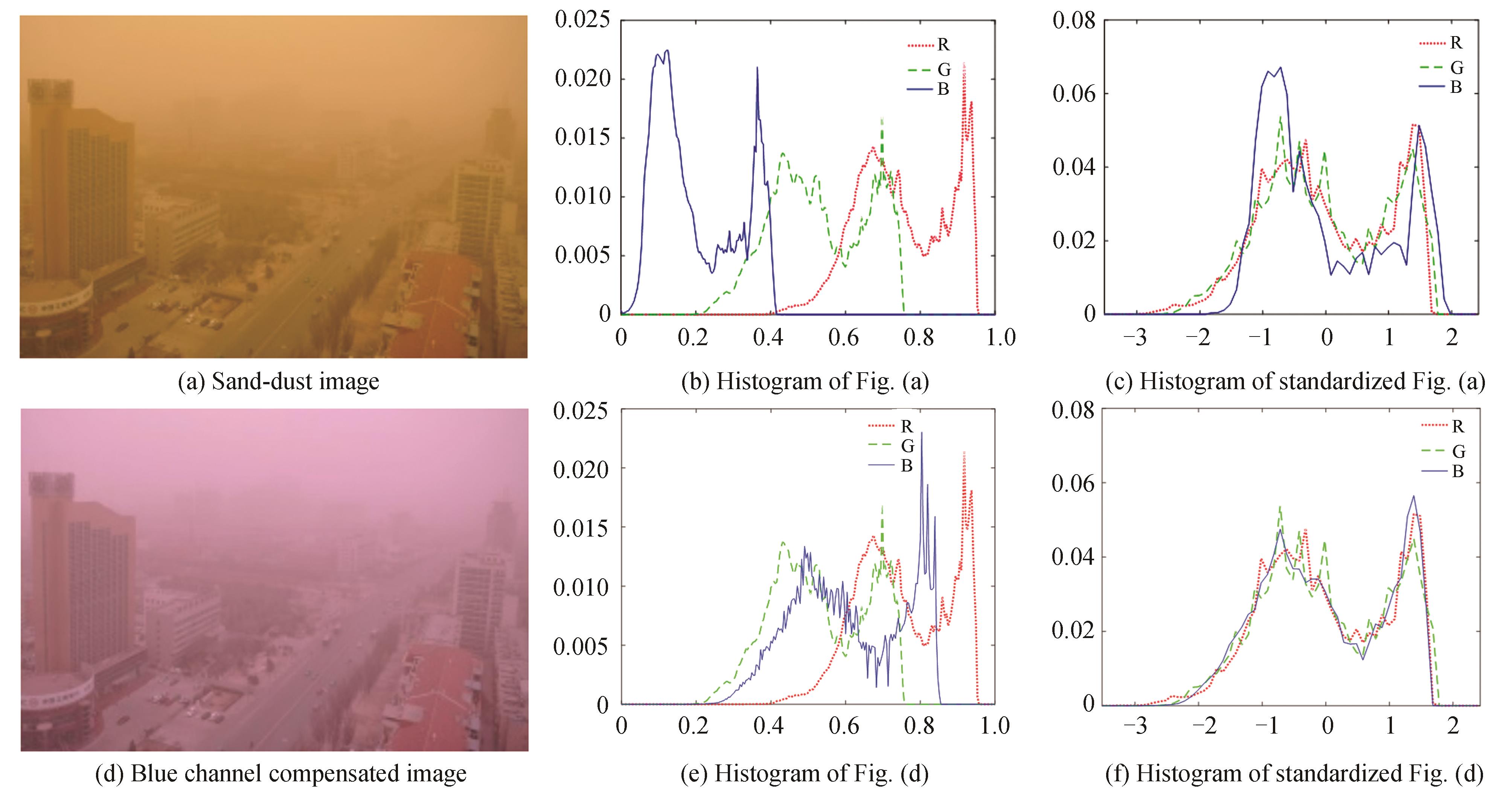
Fig. 2. The histogram of sand-dust image before and after blue channel compensation and the histogram of corresponding image standardization
Fig. 3. The enhancement results of the proposed algorithm to the sand-dust image (Fig. 2(a)) at different values of
α![]()
![]()
Fig. 4. The enhancement results of the proposed algorithm to the sand image at different values of
AB![]()
![]()
(
A![]()
![]()
=0.5)
Fig. 5. The enhancement results of the proposed algorithm to the sand image at different values of
A![]()
![]()
(
AB![]()
![]()
=0.5)
Fig. 6. Exposure images generated by the proposed algorithm and fusion result
Fig. 7. Comparison of algorithm results (Ⅰ)
Fig. 8. Comparison of algorithm results (Ⅱ)
Fig. 9. Comparison of algorithm results (Ⅲ)
Fig. 10. Comparison of algorithm results (Ⅳ)
Fig. 11. Comparison of algorithm results (Ⅴ)
Fig. 12. Comparison of algorithm results (Ⅵ)
| Orig. | Ref.[4] | Ref.[13] | Ref.[1] | Ref.[3] | Ref.[10] | Ref.[8] | Ours |
|---|
| Fig.7 | 4.126 8 | 4.004 9 | 6.110 6 | 7.793 2 | 6.005 6 | 5.935 0 | 8.353 4 | 9.176 2 | | Fig.8 | 1.504 3 | 2.879 1 | 2.687 4 | 4.006 2 | 2.488 0 | 2.685 2 | 4.791 9 | 5.605 6 | | Fig.9 | 1.652 7 | 2.413 9 | 3.300 5 | 4.580 0 | 4.472 6 | 3.309 9 | 4.780 5 | 6.366 8 | | Fig.10 | 2.560 9 | 2.401 4 | 5.571 7 | 5.051 7 | 4.512 9 | 4.187 2 | 4.613 9 | 6.063 3 | | Fig.11 | 4.392 0 | 4.195 8 | 6.931 0 | 8.029 2 | 7.255 8 | 5.664 5 | 7.776 6 | 9.558 9 | | Fig.12 | 2.074 7 | 2.548 9 | 3.045 1 | 4.531 6 | 3.882 2 | 4.939 2 | 4.594 8 | 6.331 2 | | Average | 2.718 6 | 3.074 0 | 4.607 7 | 5.665 3 | 4.769 5 | 4.453 5 | 5.818 5 | 7.183 7 |
|
Table 1. Comparison of average gradient
| Orig. | Ref.[4] | Ref.[13] | Ref.[1] | Ref.[3] | Ref.[10] | Ref.[8] | Ours |
|---|
| Fig.7 | 15.325 6 | 14.512 5 | 20.658 3 | 27.810 1 | 23.087 0 | 22.870 5 | 30.658 9 | 31.381 8 | | Fig.8 | 4.121 6 | 7.669 4 | 6.565 0 | 10.166 0 | 6.656 5 | 7.265 4 | 12.748 5 | 14.211 0 | | Fig.9 | 5.577 3 | 7.222 0 | 11.130 9 | 14.865 7 | 15.739 7 | 10.886 7 | 15.419 2 | 20.810 1 | | Fig.10 | 9.569 8 | 8.255 5 | 20.079 1 | 19.013 7 | 17.827 4 | 16.394 1 | 16.946 3 | 22.551 8 | | Fig.11 | 13.744 7 | 13.753 9 | 21.023 9 | 24.644 9 | 23.756 1 | 19.155 7 | 25.715 6 | 28.868 5 | | Fig.12 | 6.647 0 | 7.792 6 | 8.604 5 | 13.608 0 | 12.583 0 | 15.798 9 | 13.866 3 | 18.065 0 | | Average | 9.164 3 | 9.867 6 | 14.676 9 | 18.351 4 | 16.608 3 | 15.395 2 | 19.225 8 | 22.648 0 |
|
Table 2. Comparison of spatial frequency
| Orig. | Ref.[4] | Ref.[13] | Ref.[1] | Ref.[3] | Ref.[10] | Ref.[8] | Ours |
|---|
| Fig.7 | 117.616 8 | 105.468 3 | 213.710 6 | 387.295 3 | 266.914 8 | 261.930 7 | 470.707 5 | 493.164 5 | | Fig.8 | 8.499 9 | 29.431 1 | 21.565 6 | 51.711 8 | 22.170 7 | 26.412 5 | 81.321 3 | 101.049 5 | | Fig.9 | 15.574 9 | 26.114 9 | 62.034 7 | 110.647 7 | 124.041 6 | 59.342 7 | 119.041 6 | 216.830 7 | | Fig.10 | 45.886 6 | 34.147 8 | 202.006 4 | 181.138 3 | 159.239 0 | 134.663 4 | 143.888 9 | 254.821 7 | | Fig.11 | 94.700 1 | 94.826 5 | 221.568 3 | 304.463 8 | 282.898 9 | 183.940 3 | 331.492 5 | 417.762 1 | | Fig.12 | 22.133 4 | 30.420 5 | 37.090 0 | 92.765 9 | 79.317 5 | 125.041 3 | 96.321 2 | 163.483 9 | | Average | 50.735 3 | 53.401 5 | 126.329 3 | 188.003 8 | 155.763 8 | 131.888 5 | 207.128 8 | 274.518 7 |
|
Table 3. Comparison of contrast
| Process | Complexity | Process | Complexity |
|---|
| Blue channel compensation | ![]() ![]() | Construction of Gaussian pyramid | ![]() ![]() | | Image standardization | ![]() ![]() | Construction of Laplacian pyramid | ![]() ![]() | | Generation of exposure images | ![]() ![]() | Image pyramid fusion and reconstruction | ![]() ![]() | | Calculation of weight maps | ![]() ![]() | Proposed method | ![]() ![]() |
|
Table 4. Time complexity of the proposed algorithm
| Resolution | Ref.[4] | Ref.[13] | Ref.[1] | Ref.[3] | Ref.[10] | Ref.[8] | Ours |
|---|
| Fig.7 | 893×513 | 5.40 | 3.02 | 2.51 | 1.45 | 4.93 | 4.29 | 2.40 | | Fig.8 | 1 600×1 200 | 22.12 | 10.84 | 8.63 | 6.70 | 18.99 | 23.53 | 12.41 | | Fig.9 | 900×600 | 6.29 | 3.63 | 2.74 | 1.62 | 5.03 | 4.31 | 2.97 | | Fig.10 | 600×400 | 2.91 | 1.91 | 1.39 | 0.98 | 2.68 | 2.26 | 1.33 | | Fig.11 | 490×326 | 2.04 | 1.43 | 1.09 | 0.85 | 1.88 | 1.99 | 1.22 | | Fig.12 | 640×442 | 3.45 | 1.99 | 1.66 | 1.06 | 2.94 | 2.57 | 1.95 | | Total | - | 42.21 | 22.82 | 18.02 | 12.66 | 36.45 | 38.95 | 22.28 |
|
Table 5. Comparison of running time (s)