
Mariam Algarni, Kamal Berrada, Sayed Abdel-Khalek. Atom-field system: Effects of squeezing and intensity dependent coupling on the quantum coherence and nonclassical properties[J]. Journal of the European Optical Society-Rapid Publications, 2023, 19(2): 2023039
Journals >Journal of the European Optical Society-Rapid Publications >Volume 19 >Issue 2 >Page 2023039 > Article
- Journal of the European Optical Society-Rapid Publications
- Vol. 19, Issue 2, 2023039 (2023)
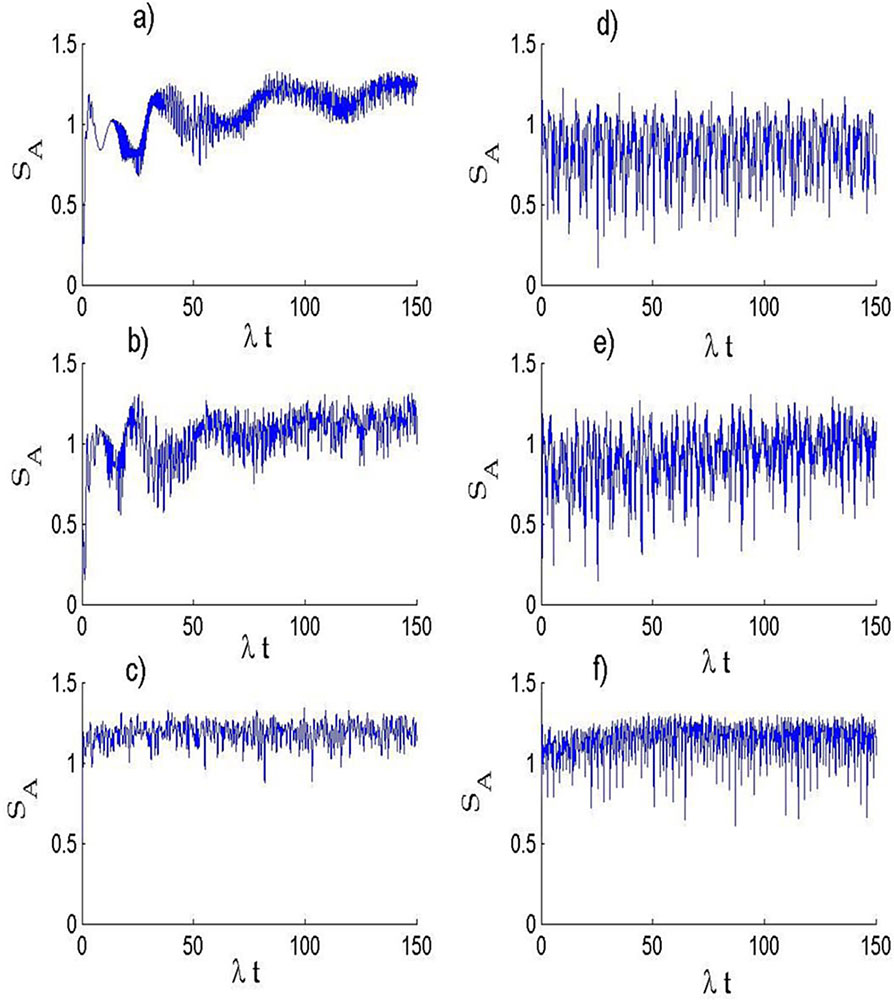
Fig. 1. Temporal evolution of
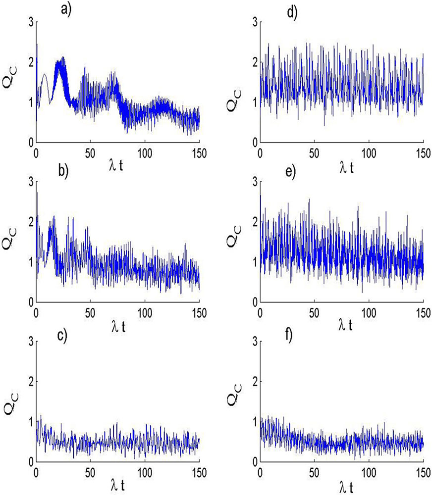
Fig. 2. Temporal evolution of
Fig. 3. Temporal evolution of QM for the field initially prepared in a SCS with |α|2 = 25. The subfigures (a, b, c) are for

Set citation alerts for the article
Please enter your email address
© Copyright 2018-2021 | Chinese Laser Press. All Rights Reserved 沪ICP备15018463号-20