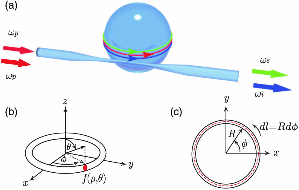
Fig. 1. (a) Schematic of an SFWM photon pair source based on a fused silica microsphere, evanescently coupled to a fiber taper placed in closed proximity; (b) transverse mode of propagation around the sphere perimeter; (c) top view of the guided mode.

Fig. 2. (a) and (b) Density plots of the phase-matching function |sinc(LΔκl→pl→s)l→i(ωp,Ω)/2)|2; also shown are the specific contours defined by LΔk=0 and LΔk=0.49 [which correspond to sinc(LΔk/2) equal to 1 and 0.99, respectively], for a sphere with R=135  μm, for two values of Q, as indicated. The black rectangle indicates the region of interest in our experiments, centered around 1550 nm. (c) and (d) Plots similar to (a) and (b), for Q=108 and much larger radii (R=1.35  cm and R=1.35  m).

Fig. 3. (a) FSR versus optical frequency, calculated from Eq. (4); (b) and (c) sketch of generation-mode matrix assuming a constant FSR, plotted versus ωs and ωi [in panel (b)], and versus Ω and ω+ [in panel (c)]; (d) and (e) sketch of generation-mode matrix assuming an FSR with spectral drift, plotted versus ωs and ωi [in panel (d)], and versus Ω and ω+ [in panel (e)].

Fig. 4. For a microsphere with radius R=135  μm and Qs=Qi=1×108, two-dimensional plot of the joint SI [computed from Eq. (25)], plotted within a region of 300 MHz width, centered at each point of the generation mode-matrix main diagonal (with a separation of 1.52 THz between regions along ωs,i); inset, close-up of central region, corresponding to ls=li=774.

Fig. 5. This figure clarifies the structure of the two-photon state produced by SFWM in a microsphere device, in regions similar to those defined in Fig. 4 for the same source, in the frequency variables Ω and ω+. We show plots of the function As(ω++Ω), Ai(ω+−Ω), As(ω++Ω)Ai(ω+−Ω), and As(ω++Ω)Ai(ω+−Ω)Ap(ω+) in each of rows (a) through (d). Note that in (c) we have indicated with a pair of dotted lines the spectral width of the pump resonance. In (e), we show a plot of the function Ri(Ω), obtained by integrating As(ω++Ω)Ai(ω+−Ω)Ap(ω+) over ω+ [or equivalently over ωp; see Eq. (31)], yielding the idler-photon SI in the form of a frequency comb.

Fig. 6. In this figure, we show the behavior of the idler-photon SI Ri(Ω), for the same source as assumed in the previous two figures [computed from Eq. (31); see also Fig. 5], for three different values of the Q coefficients [Q = 10⁸ in (a), Q = 10⁷ in (b), and Q = 10⁶ in (c)], assumed to be the same for both signal and idler modes.

Fig. 7. In panels (a)–(c) of this figure, we show plots of the TED function R˜(T) (with T=ts−ti), obtained for the same source as assumed for Figs. 6(a)–6(c), for three different values of Q=Qs=Qi. (d) Close-up around the central region of the plot in (a), showing the temporal oscillations with period equal to the cavity round-trip time, which cannot be resolved in panels (a)–(c).

Fig. 8. (a) Experimental setup. LC, laser controller; DWDM, dense wavelength division multiplexing device; EDFA, erbium-doped fiber amplifier; PC, polarization controller; TF, tapered fiber; MS, microsphere; CWDM, coarse wavelength division multiplexing device; MC, grating-based monochromator; ID230, free-running InGaAs APD; ID800, time-to-digital converter. Note that in some of the subsequent figures we have provided a setup sketch to show variations on the setup shown in this figure. (b) Close-up showing the fiber taper-microsphere system; (c) schematic of source operation and data obtained in our measurements.

Fig. 9. Experimentally obtained normalized transmittance reduction versus ω (calculated as the difference between transmission far from the resonance and the transmittance at each ω), for a particular cavity resonance, shown together with an Airy function Ap(ω) fit.

Fig. 10. (a) Sketch of the experimental setup used for the characterization of the signal-idler SFWM spectrum; (b) SFWM spectrum, composed of pairs of energy-conserving peaks, also showing regions colored red, green, and blue, indicating each of three relevant CWDM channels. We have included the measured transmission curves for these three CWDM channels. (c) For the signal photon, i.e., corresponding to λ<λp, the individual emission peaks (shown using a logarithmic scale), along with a map of the DWDM channels used, including the transmission curves for each of these channels.

Fig. 11. (a) Sketch of the setup used for the results shown in (b) and (c); (b) isolation of tallest pair of energy-conserving peaks from Fig. 10(a), obtained by filtering the signal photon with a DWDM channel and the idler photon with a grating monochromator; (c) total SFWM flux, integrated within the signal-mode peak in (b), as a function of pump power, along with a quadratic fit; (d) sketch of the setup used for the results shown in (e); (e) coincidence count rate as a function of the detection time difference between the signal and idler modes, presenting a well-defined peak near zero delay; inset, peak close-up; (f) sketch of the setup used for the results shown in (g); (g) similar to panel (e), but the signal photon is transmitted through a 12.8 km stretch of fiber.

Fig. 12. For a microsphere with R=180  μm, the pump transmitted through DWDM channel 33, and the signal photon transmitted through DWDM channel 47. (a) Heralded idler photon emission characteristics in the space formed by the idler wavelength λi and the signal-idler time of detection difference T=ts−ti; (b) marginal distribution in λi; (c) marginal distribution in variable T; (d) graphical representation of wavelengths involved for the pump, signal, and idler modes, for idler frequency denoted by red arrow in (a); (e) measured TED; (f) inferred idler-mode single-photon intensity spectral distribution. Panels (g)–(l) are similar to panels (a)–(f), except that DWDM channel 49 is used, instead of 47, to transmit the signal photon. For a microsphere with R=180  μm, the pump is transmitted through DWDM channel 34, and the signal photon is transmitted through DWDM channel 48. (m) Heralded idler photon emission characteristics in the space formed by the idler wavelength λi and the signal-idler time of emission difference T; (n) marginal distribution in λi; (o) marginal distribution in variable T; (p) graphical representation of wavelengths involved for the pump, signal, and idler modes, for idler frequency denoted by red arrow in (m); (q) measured time of emission difference distribution; (r) inferred idler-mode single-photon intensity spectral distribution; panels (s)–(x) are similar to panels (m)–(r), except that DWDM channel 49 is used, instead of 48, to transmit the signal photon.

Fig. 13. For a microsphere with R=135  μm, and the pump transmitted through DWDM channel 33, (a) and (d) show the idler mode, single-photon emission characteristics for narrowband filtering (DWDM channel 48) in (a), and for wideband filtering [1530 nm CWDM channel in (d)]. Panels (b) and (e) show spectral marginal distributions for the distributions in (a) and (d), respectively. Panel (c) shows a temporal marginal distribution for the distribution in (a).

Table 1. Details of the Various Experimental Runs Shown in Figs. 12 and 13^a