Fig. 1. Schematic diagram for absolute instability regions due to (a) the second-order rescattering of SRS and (b) the third-order rescattering of SRS in a linearly inhomogeneous plasma with density $[0.01,0.2]n_{c}$. BSRS means backscattering of SRS.

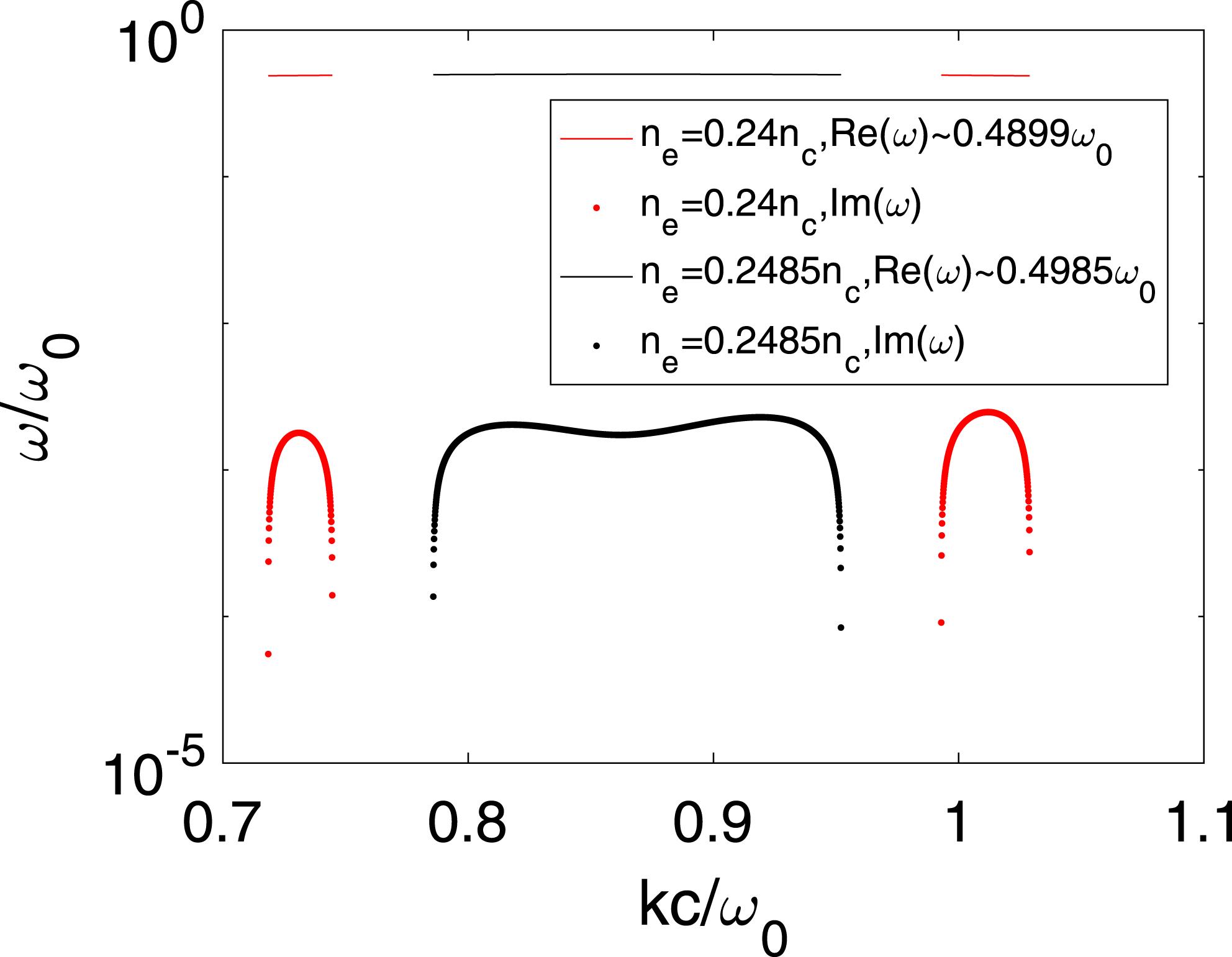
Fig. 2. Numerical solutions of SRS dispersion equation at the plasma density $n_{e}=0.24n_{c}$ and $n_{e}=0.2485n_{c}$, where $a_{0}=0.01$. The dotted line and continuous line are the imaginary part and the real part of the solutions, respectively.

Fig. 3. PIC simulation results for the development of the absolute SRS via the second-order scattering. (a) and (b) Wavenumber–frequency distributions of the scattered light in the time windows $[1501,2000]\unicode[STIX]{x1D70F}$ and $[2001,2500]\unicode[STIX]{x1D70F}$, respectively. FSRS means forward scattering of SRS. (c) 2D Fourier transform $|E_{L}(k,\unicode[STIX]{x1D714})|$ of the electric field in the time window $[2001,2500]\unicode[STIX]{x1D70F}$. (d) Fourier spectra of backscattered light diagnosed at $x=10\unicode[STIX]{x1D706}$. (e) Time–space distributions of Langmuir waves, where $E_{L}$ is the longitudinal electric field normalized by $m_{e}\unicode[STIX]{x1D714}_{0}c/e$, $m_{e}$, $c$ and $e$ are electron mass, light speed in vacuum and electron charge, respectively. (f) Longitudinal velocity distributions of electron at different time. (g) Longitudinal phase space distribution of electrons near the region of the absolute SRS instability at $t=3250\unicode[STIX]{x1D70F}$. (h) Energy distributions of electrons at different time, where $N_{e}$ is the relative electron number.

Fig. 4. The case when the absolute SRS is absent provided $n_{\text{min}}>n_{c}/9$. (a) Wavenumber–frequency distributions of the scattered light in the time window $[2001,2500]\unicode[STIX]{x1D70F}$. (b) Energy distributions of electrons at different time.

Fig. 5. (a)–(c) PIC simulation results for a plasma at $T_{e0}=1$ keV with immovable ions. (a) 2D Fourier transform $|E_{L}(k,\unicode[STIX]{x1D714})|$ of the electric field in the time window $[2001,2500]\unicode[STIX]{x1D70F}$. (b) Time–space distributions of Langmuir waves. (c) Longitudinal phase space distribution of electrons at $t=2800\unicode[STIX]{x1D70F}$. (d) Energy distributions of electrons with different temperatures or different ions at $t=4000\unicode[STIX]{x1D70F}$.

Fig. 6. Development of absolute SRS instability as seen from 2D PIC simulation with $a_{0}=0.02$ and $T_{e0}=2$ keV. The incident laser is p-polarized. (a) Spatial Fourier transform $|E_{L}(k_{x},k_{y})|$ of the electric field at $t=2300\unicode[STIX]{x1D70F}$. (b) Energy distributions of electrons at different time.

Fig. 7. PIC simulation results for the development of the absolute SRS via the third-order scattering. (a)–(c) Simulation results for the plasma with the inhomogeneous plasma density range $[0.04,0.09]n_{c}$. (a) and (b) show the 2D Fourier transform $|E_{s}(k,\unicode[STIX]{x1D714})|$ of the scattered light $E_{s}(x,t)$ in the time windows $[3001,4000]\unicode[STIX]{x1D70F}$ and $[4001,5000]\unicode[STIX]{x1D70F}$, respectively. (c) 2D Fourier transform $|E_{L}(k,\unicode[STIX]{x1D714})|$ of the electric field in the time window $[5001,6000]\unicode[STIX]{x1D70F}$. The white line denotes the linear resonant region for convective backscattering SRS. (d) 2D Fourier transform $|E_{L}(k,\unicode[STIX]{x1D714})|$ of the electric field in the time window $[5001,6000]\unicode[STIX]{x1D70F}$, when the plasma density profile is limited to the range of $[0.0625,0.09]n_{c}$.