In indirect-drive inertial confinement fusion (ICF),¹ hohlraum targets made of high-Z material are employed to convert the incident laser energy to X rays to drive the implosion, and, for symmetry control, the hohlraum is commonly filled with a low-Z gas to suppress the expansion of the high-Z plasma from the hohlraum wall. Therefore, for an ignition hohlraum, the internal plasma conditions are quite complex, with plasmas generated from the hohlraum wall, the infill gas, and the ablator of the fuel pellet interacting with each other. Owing to these complex and unexpected internal plasma conditions, problems connected with laser plasma interaction (LPI)² are among the most serious that arise in attempts to achieve ignition, and they remain unsolved in the National Ignition Campaign (NIC)³ conducted on the National Ignition Facility (NIF),⁴ the largest ICF laser facility in the world at present. To improve hohlraum performance, it is essential to gain a better understanding of laser–hohlraum energy coupling and the relevant physics concerning LPI, energy deposition, and X-ray conversion. To achieve this, the internal plasma conditions need to be precisely diagnosed experimentally, and the dynamic and kinetic effects relevant to hohlraum plasma evolution need to be thoroughly investigated. However, measurement of hohlraum plasma conditions is quite challenging, owing to the complex experimental environment on large laser facilities and the closed geometry of hohlraum targets. Therefore, it is critical to develop an appropriate diagnostic for hohlraum plasma conditions.

Among the various plasma diagnostic methods that are available, optical Thomson scattering (OTS)⁵ is one of the best choices, since it is capable of providing unperturbed, local, and precise measurements.^6,7 OTS diagnostic measures the scattering spectra of an incident laser by free electrons within a plasma, which directly reflect electron motion and are sensitive to intrinsic plasma density fluctuations. With an appropriate experimental design, OTS can diagnose a variety of plasma parameters,^6–9 including the electron temperature, the electron density, the plasma flow velocity, the ion temperature, the averaged ionization state, and the ion species fraction. Hence, applying OTS to ICF hohlraums will greatly enhance diagnostic capacity and help to understand hohlraum plasma behavior. However, despite the advantages of OTS in plasma characterization, its experimental implementation is still challenging. The primary reason is that the Thomson scattering cross section is quite small—under typical conditions, the intensity of the scattered light is nine orders of magnitude weaker than that of the incident light. Therefore, a high-energy probe beam is often required, and the experimental setup needs to be very carefully designed to avoid strong background noise and obtain an acceptable signal-to-noise ratio.

Throughout the development of the OTS diagnostic for ICF purposes, research groups in the United States have made a remarkable contribution. The first Thomson scattering experiment for ICF hohlraum targets was conducted on the NOVA laser facility¹⁰ with a 2ω (526.6 nm) probe laser, and the electron temperature, ion temperature, and plasma flow velocity in the gas-filled region were measured. Subsequently, the OTS diagnostic was upgraded, with the use of a 4ω (263.3 nm) probe laser.¹¹ For this wavelength band, there is less light absorption in the plasma, and the critical density is higher, which allows measurements to be made in higher-density regions. In addition, the background noise of stimulated Raman side scattering from the 3ω (351 nm) drive beams can be avoided. Since then, 4ω probe lasers have been commonly used for ICF hohlraums, and OTS has been continuously developed on the OMEGA laser facility,¹² where multicolor Thomson scattering¹³ and imaging Thomson scattering¹⁴ were implemented. To further reduce background noise from 3ω drive beams in an ignition-scale hohlraum, a 5ω (210 nm) OTS diagnostic has also been designed on the NIF,¹⁵ which is quite challenging for deep-ultraviolet optical transmission and detection.

In China, we have also developed OTS diagnostics for ICF research. Early experiments were conducted on the Xingguang-II laser facility¹⁶ with a 2ω probe beam and on the Shenguang-II laser facility^17,18 with a 4ω probe beam. They focused mainly on targets with open geometry, such as disk targets and gas-bag targets, which provide simpler plasma conditions than hohlraums. These early explorations have played an important role in understanding the behavior of laser-produced plasmas and have paved the way for OTS experiments with hohlraum targets. In recent years, 4ω OTS diagnostics have been successively implemented on 10 kJ-level¹⁹ and 100 kJ-level²⁰ laser facilities, and our research focus has been on the internal plasma conditions of gas-filled hohlraums. To reduce the complexity of hohlraum plasma conditions in the preliminary study, we have adopted hohlraums without any pellets inside. To establish the predictive capability of our experiments, we have developed a method to simulate time-resolved Thomson scattering spectra, where the input plasma conditions are given by the 2D radiation-hydrodynamic code LARED.²¹ The simulated spectra can provide guidance for experimental measurements and can be compared directly with the measured spectra. To analyze the accuracy of measurement of plasma parameters, we have also explored the fitting method for Thomson scattering spectra. Recent experiments have involved different types of hohlraums. A typical experiment with a simplified cylindrical hohlraum has been conducted on the 10 kJ-level laser facility, where the geometry was kept quasi-2D to facilitate comparisons with simulations. The plasma evolution around the laser entrance hole (LEH) has been studied, and the experimental results are in good agreement with the simulations. The dynamic effects of the blast wave generated from the covering membrane and the convergence of shocks on the hohlraum axis have been observed. Another experiment with an octahedral spherical hohlraum²² has been conducted on the 100 kJ-level laser facility, and the plasma evolution at the center of the hohlraum has been studied. A major discrepancy appears between experiment and simulation as the electron temperature rises, indicating the occurrence of nonlocal thermal conduction, which has not been considered in the simulation code.

In this paper, we briefly review progress in recent explorations of the measurement of internal plasma conditions in gas-filled hohlraums. In Sec. II, we present the model for the Thomson scattering spectra calculation, including spectral fitting of experimental data and spectral simulation based on LARED, which are two helpful ways to understand the behavior of hohlraum plasmas. In Sec. III, we describe the experiment on the simplified cylindrical hohlraum, and discuss the plasma evolution in the LEH region. In Sec. IV, we describe the experiment on the octahedral spherical hohlraum, and discuss the plasma conditions at the hohlraum center. Section V is a summary.

For a probe laser with intensity I₀, frequency ω_i, and wave vector k_i, the power of Thomson-scattered light with wave vector k_s in solid angle dΩ and in the frequency range from ω_s to ω_s + dω is⁵PsdΩdω=12πI0re2Vne(1+2ωωi)sin2⁡φS(k,ω)dΩdω,(1)where ω = ω_s − ω_i and k = k_s − k_i are the frequency and wave vector of the probed mode of plasma density fluctuations, r_e is the classical electron radius, V is the scattering volume, n_e is the electron number density, φ is the angle between the polarization direction of the incident light and the propagation direction of the scattered light, and S(k, ω) is the spectral density function.

The spectral density function S(k, ω) for plasmas with multiple ion species can be expressed as⁵S(k,ω)=2πk|1−χeϵ|2fe0(ωk)+2πk|χeϵ|2∑jZj2Nj∑jZjNjfi0,j(ωk),(2)where the subscript j stands for the jth ion species, Z_j is the ion charge, N_j is the ion number density, χ_e (χ_j) and f_e0 (f_i0,j) are the electron (ion) susceptibility and the normalized 1D electron (ion) velocity distribution function, respectively, and ϵ=1+χe+∑jχj is the plasma dielectric function.

The scattering parameter is defined as α ≡ 1/kλ_De, where λ_De is the Debye length. When α > 1, collective scattering from intrinsic plasma wave modes dominates, and resonant features related to ion-acoustic waves (IAWs) and electron plasma waves (EPWs) can be observed in the scattered spectra. For measurement at a specific scattering angle, the plasma waves co- and counter-propagating along k are probed, and the frequency differences between the scattered and the incident light in the laboratory frame are determined by the frequencies of plasma waves and the Doppler shift caused by plasma flow,⁷ which areΔω±IAW=±ωIAW+(ks−ki)⋅u=±kcs+k⋅u(3)for the IAW features andΔω±EPW=±ωEPW+(ks−ki)⋅u=±ωpe2+3k2vte2+k⋅u(4)for the EPW features, where Δω_± correspond to the blue- and red-shifted resonant features, u is the plasma flow velocity, cs≅(ZTe+3Ti)/mi is the ion sound speed (T_e and T_i are the electron and ion temperatures, and m_i is the ion mass), ω_pe is the plasma frequency, and v_te is the root-mean-square (rms) thermal speed of electrons. Equations (3) and (4) show that the IAW features are sensitive to ZT_e, T_i, and u, while the EPW features are mainly sensitive to n_e, since the dominant term in Eq. (4) is ωpe2∝ne. In practice, the plasma parameters are obtained by fitting the spectra calculated with Eqs. (1) and (2) to those measured by experiment.

In spectral fitting for high-temperature (>1 keV) hohlraum plasmas, the Thomson scattering theory of collisionless, unmagnetized plasmas with Maxwellian distributions is most commonly used. For Maxwellian distributions, the functions f_e0 and f_i0,j in Eq. (2) take the formsfe0(v)=12πvteexp(−v22vte2),(5)fi0,j(v)=12πvtjexp(−v22vtj2),(6)where v_te and v_tj are the rms thermal speeds of electrons and the jth species of ions, respectively, and the electron and ion susceptibilities χ_e and χ_j in Eq. (2) take the formsχe(k,ω)=α2w(xe),(7)χj(k,ω)=α2Zj2Nj∑jZjNjTeTjw(xj),(8)where xe=ω/(2kvte), xj=ω/(2kvtj), andw(x)=1−2xe−x2∫0xep2dp+iπxe−x2.(9)When dealing with collisional effects²³ or non-Maxwellian distributions,²⁴ the expressions above for susceptibilities and distribution functions should be modified.

Least-squares fitting is performed to infer the plasma parameters from the experimental data. The problem can be described as finding the input X that minimizes the quantityr≡∑λ[Pfit(λ,X)−Pexp(λ)]2,where X represents the parameters to be inferred, λ is the measured wavelength corresponding to the camera pixels, and P_fit and P_exp are the calculated and measured Thomson scattering power spectra, respectively. Generally, the input X for the IAW features contains the electron temperature T_e, the ion temperature T_i, the plasma flow velocity u, and the electron drift velocity u_d, where u contributes to the Doppler shift, while u_d contributes to the difference in Landau damping and thus the asymmetry of the blueshifted and redshifted features. These velocities are included in the calculation by substituting ω = ω_s − ω_i − k · u into f_i0 and χ_i, while substituting ω = ω_s − ω_i − k · (u + u_d) into f_e0 and χ_e in Eqs. (5)–(9). Other parameters required in the calculation, such as the electron density and the ion charge, are assumed in the fitting for the IAW features.

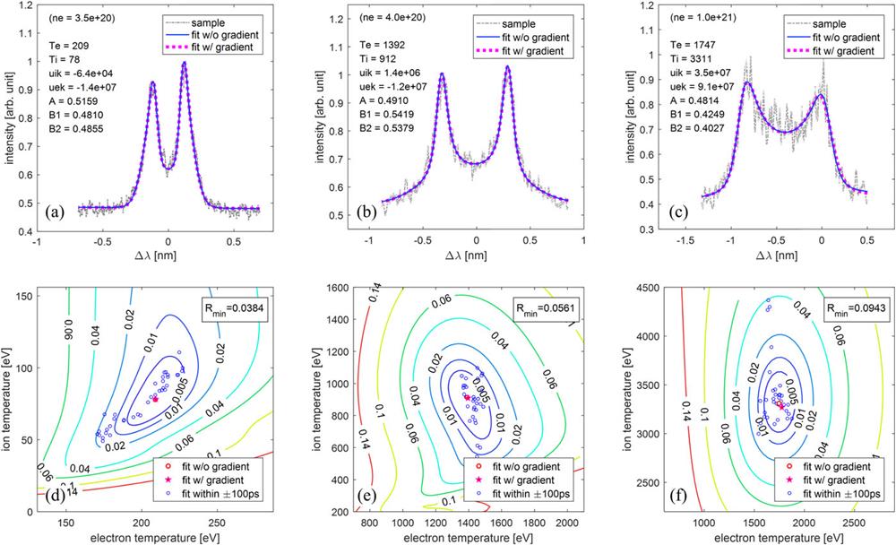
When calculating P_fit, the instrumental effects (spectral response and resolution) and the background noise in the experiment should be taken into account. For the IAW features, the background can be approximated as linear in spectrum, and P_fit can be written asPfit(λ,X)=APsignal(λ,Te,Ti,uik,uek)+B1+B2−B1λ2−λ1(λ−λ1),(10)where P_signal is normalized by its maximum, A is the relative amplitude of the signal, B₁ and B₂ are the relative background levels at the two sampled ends λ₁ and λ₂, respectively, u_ik ≡ k·u, and u_ek ≡ k · (u + u_d). Hence, X involves seven variables (T_e, T_i, u_ik, u_ek, A, B₁, B₂) to be fitted. Figures 1(a)–1(c) show three examples of the spectral fitting, with different temperature levels. The samples in Figs. 1(a) and 1(b) are extracted from the data from the octahedral spherical hohlraum experiment [see Sec. IV, Fig. 10(a); the samples are taken at 2 ns and 4.3 ns, respectively], while the sample in Fig. 1(c) is extracted from the data from the cylindrical hohlraum experiment [see Sec. III, Fig. 5(a); the sample is taken at 2.2 ns].

To evaluate the uncertainty of the fitting process, we can consider the quantityR≡1AfitrN,where r is the sum of squares defined above, N is the total number of terms in the summation, and A_fit is the best-fit signal amplitude corresponding to the A in Eq. (10). By definition, R reaches a minimum at the best-fit point, and R_min characterizes the noise-to-signal ratio in the fitting process. Figures 1(d)–1(f) show the contours of the difference ΔR = R − R_min around the best-fit point in the T_e–T_i plane, corresponding to Figs. 1(a)–1(c), respectively. These contours reflect the parameter sensitivities and can be used to estimate the fitting uncertainty. For instance, taking the contours of 0.005 in Figs. 1(d)–1(f), the relative uncertainties for electron (ion) temperature are estimated to be ±9% (±30%), ±10% (±24%), and ±9% (±10%), respectively.

As a comparison, the best-fit points of different spectrum samples within ±100 ps are shown in these contour maps. In practice, each sample is extracted from a one-pixel time interval of the original spectral image. The fluctuation of the best-fit points can also be used to estimate the fitting uncertainty, since the plasma parameters vary slightly within ±100 ps. Taking the standard deviation of these points in Figs. 1(d)–1(f), the relative uncertainties for electron (ion) temperature are estimated to be ±9% (±22%), ±3% (±15%), and ±5% (±10%), respectively, which are within the uncertainties estimated by the contours mentioned above.

For further evaluation, the effects of plasma gradients and k-vector smearing should be considered. However, for the discussion in this paper, the k-vector smearing effect is quite small, since the scattered light is collected in an f/10 cone and the k variance is only about ±2.5%. The fitting results considering these two effects are also shown in Figs. 1(d)–1(f). The plasma gradients in the fitting process are given by radiation-hydrodynamic simulations. In Figs. 1(d) and 1(e), the gradients are small, with a T_e variation of ±5% and a T_i variation of ±10%, and thus the best-fit points almost coincide with those obtained without considering gradients. In Fig. 1(f), the gradients are larger, with a T_e variation of ±5%, a T_i variation of ±20%, and a u_ik variation of ±12%. As a result, the best-fit point shifts a little, but is still close to the point without gradient.

In addition, the pre-assumption of electron density also has an influence on the fitting result. Figure 2 shows the variation of the best-fit temperatures when assuming different electron densities in the fitting process. The corresponding spectrum is the one shown in Fig. 1(b). According to simulation, the electron density within the Thomson scattering volume varies from 3 × 10²⁰ to 5 × 10²⁰ cm⁻³, as shown in the shaded area of Fig. 2. Therefore, the uncertainties in the electron (ion) temperature induced by the density assumption are estimated to be ±6% (±1%). For a general consideration, a Monte Carlo approach can be applied in error analysis.⁷

The aim of Thomson scattering spectral simulation is to build up the predictive capability for experiments, which contributes to experimental design and data analysis. The spectra are calculated according to Eqs. (1)–(9), using the plasma conditions given by the 2D radiation-hydrodynamic code LARED.²¹

Figure 3(a) shows an example of simulation with cylindrical symmetry, where the Z direction is along the hohlraum axis and the R direction is along the hohlraum radius. The Thomson scattering volume is defined by the overlap of the probe beam and the diagnostic aperture, as shown in Fig. 3(b), where the whole scattering volume is divided into a number of volume elements for consideration of plasma inhomogeneity. Each element is assigned a 2D coordinate (Z, R) and a set of plasma parameters (T_e, T_i, n_e, etc.) corresponding to the positions in the simulation, and the Thomson scattering spectra at each volume element are calculated separately and then summed. The solid angle dΩ in Eq. (1) is determined by the f-number F of the collecting optics. For the f/10 collection system used in our experiments, the solid angle is quite small and can be approximated as dΩ ≅ π/(4F²). The spectral response, the spectral resolution, and the inverse bremsstrahlung absorption²⁵ along the optical path are also involved in the calculation. Finally, the spectra calculated at different time are synthesized as time-resolved spectra, with temporal resolution accounted for.

In this section, we review a typical experiment with a simplified cylindrical hohlraum, as shown in Fig. 4. The target is a cylindrical gold hohlraum with two open ends as LEHs, and both the diameter and the length of the hohlraum are 1.4 mm. The hohlraum is filled with pentane (C₅H₁₂) gas at a pressure of 0.6 atm, corresponding to an electron density of 6 × 10²⁰ cm⁻³ when fully ionized. Seven 3ω (351 nm) heater beams penetrate the hohlraum through both ends, with an angle of 45° relative to the hohlraum axis, delivering a total energy of 5.6 kJ in 2 ns main pulse plus a 0.5 ns pre-pulse. The heater beams are smoothed by continuous phase plates (CPPs), with 500 μm-diameter focal spots in the LEH plane. To retain a quasi-2D geometry, the laser spots on the hohlraum wall are arranged in a single ring in the equatorial plane. The 4ω (263.3 nm) probe beam is aligned horizontally and enters the hohlraum through a diagnostic hole (0.35 × 0.35 mm²) on its wall, with 90 J energy in a 3 ns pulse and a 100 μm-diameter focal spot. The probe pulse is synchronized to the heater pre-pulse, and thus is 0.5 ns ahead of the heater main pulse. The scattered light is collected downward, with a scattering angle of 90°, and the scattering volume is ∼100 × 100 × 100 µm³, defined by the probe beam and the diagnostic system. A 750 mm-spectrometer and a streak camera are used to record the IAW features of the scattered light, with a spectral resolution of 0.065 nm in full width at half maximum (FWHM).

Figures 5(a) and 5(c) show the measured Thomson scattering spectra from the positions 225 µm inside and 250 µm outside the LEH, respectively, and Figs. 5(b) and 5(d) show the simulated spectra corresponding to Figs. 5(a) and 5(c), respectively. As a rough comparison, the evolution of the IAW features measured by experiment is in accordance with simulation, except for background noise and some differences in detail. In Fig. 5(a), strong noise occurs at the beginning of the heater main pulse (t = 0.5 ns), with a bright speck near Δλ = 0 and a broadband stripe, which are probably related to stray light and the LEH covering membrane. In addition, the absence of signal before t = 0.5 ns is mainly caused by the covering membrane, which forms a plasma that is too dense to allow transmission of the incident and scattered light at an early stage. In Fig. 5(c), the absence of a signal before 0.4 ns is due to the absence of plasma before the ablated plasma expands into the Thomson scattering region.

Figure 6 shows the evolution of the electron and ion temperatures and the component of the plasma flow velocity along the k direction, corresponding to the two positions measured in the experiment. The triangles and squares with error bars are inferred from the spectra shown in Figs. 5(a) and 5(c), respectively, by the fitting method presented in Sec. II B. The lines are extracted from the radiation-hydrodynamic simulation, and the shaded areas characterize the plasma inhomogeneity within the Thomson scattering volume, as introduced in Sec. II C. As with the comparison in Fig. 5, there is also good agreement between experiment and simulation in Fig. 6.

For the position inside the LEH, the signal continues to weaken from t = 1 ns to t = 2 ns, as can be seen from Figs. 5(a) and 5(b). This is due to a shock wave (blast wave) from the LEH membrane, generated at the onset of the heater main pulse. Figure 7(a) shows simulation maps of the ion temperature and the electron density at t = 1 ns, where the two diagnosed positions are starred in red (Z = −475 and Z = −950). A shock structure propagating inward can be seen, and the shock front just reaches the position Z = −475 at this time. After the shock, a rarefaction wave follows, and the electron density continues to decrease at this position, thus accounting for the decrease in signal intensity. For the measured spectra, the signals from 1.5 ns to 2 ns are so weak that the redshifted features cannot even be recorded.

For both positions, the IAW features show a sharp twist at a late stage (see Fig. 5), which indicates a rapid change in plasma flow velocity. This change in velocity can be seen in Fig. 6(c), and is also associated with a sharp increase in ion temperature, as shown in Fig. 6(b). This behavior is due to the convergence of shock waves on the hohlraum axis. Figure 7(b) shows simulation maps of the ion temperature and electron density at t = 2 ns. A region of high T_i and high n_e forms along the hohlraum axis as the shock waves from the hohlraum wall gradually converge and squeeze the plasma out. This also accounts for the order of time for the change to occur at these two positions: for Z = −475, the change occurs at ∼2 ns, and for Z = −950, the change occurs at ∼2.7 ns.

From a more detailed comparison, it is found that there are two main differences between experiment and simulation. First, the signal intensity at a late stage given by simulation is much higher than that actually measured (see Fig. 5), which indicates that convergence of shocks leads to a higher electron density in simulation than experiment. Second, the measured flow velocity inside the LEH [see Fig. 6(c), where the negative velocity is along the −k direction] is larger than in the simulation at an early stage, thus causing a larger redshift in the spectra [see Figs. 5(a) and 5(b)]. These differences are probably caused by the asymmetries in the experiment, especially when there are only three beams heating the hohlraum from the bottom (see Fig. 4). Such asymmetries can weaken the effect of shock convergence, thus reducing the increase in electron density on the hohlraum axis. In addition, the asymmetry of the heater arrangement can also lead to a radial velocity with a component along the −k direction, which accounts for the larger redshift in Fig. 5(a).

An octahedral spherical hohlraum²⁶ is a recently conceived type of hohlraum with a better symmetry than the traditional cylindrical hohlraum and therefore promising for use in ICF ignition. The experimental capabilities of octahedral spherical hohlraums have been developed, and studies of hohlraum energetics have been carried out.²⁷ After implementation of the OTS diagnostic,²⁰ we conducted a Thomson scattering experiment to study the internal plasma conditions of a gas-filled octahedral spherical hohlraum. In this section, we describe the experiment and discuss the results of measurements at the center of the hohlraum.

Figure 8 shows the configuration of the Thomson scattering experiment with an octahedral spherical gold hohlraum (with six LEHs). The hohlraum is filled with pentane (C₅H₁₂) gas at a pressure of 0.35 atm, corresponding to an electron density of ∼3.5 × 10²⁰ cm⁻³ when fully ionized. The diameters of the hohlraum, the two polar LEHs, and the four equatorial LEHs are 4.8 mm, 1.2 mm and 1.4 mm, respectively. The laser arrangement here is similar to that in the hohlraum energetics experiment,²⁷ with 32 beams (3ω) heating the hohlraum through six LEHs, delivering a total energy of ∼80 kJ. The heater pulse is made up of a 0.5 ns pre-pulse and a 3 ns main pulse, with a 1 ns interval. The 4ω probe beam is aligned vertically and enters the hohlraum through the top LEH, with 90 J energy in a 3 ns pulse. To reduce the influence of the probe beam on the plasma states, the probe pulse is delayed by 0.3 ns relative to the heater main pulse. The scattered light is collected through an equatorial LEH, with a scattering angle of 90° and a scattering volume of ∼100 × 100 × 100 µm³. Time-resolved IAW features are measured with a 750 mm spectrometer and a streak camera, and the spectral resolution is 0.057 nm in FWHM.

In the simulations, the octahedral spherical hohlraum with six LEHs is simplified as a spherical hohlraum with two LEHs, by equating the sum of the LEH areas, as can be seen in Fig. 9, where the equivalent LEH radius is 1.16 mm. Similarly, the laser arrangement is also simplified as two cones with a single incident angle relative to the hohlraum axis. Figures 9(a) and 9(b) show maps of the electron temperature at t = 2 ns (the heater main pulse starts at t = 1.5 ns) from simulations without and with the probe beam, respectively. It can be clearly seen that the electron temperature along the laser paths is higher than in the surrounding areas and that the electron temperature along the hohlraum axis in Fig. 9(b) is higher owing to heating by the probe beam.

Figure 10(a) shows the Thomson scattering spectra measured at the hohlraum center. Owing to the geometrical symmetry, the plasma flow velocity at the hohlraum center is quite small; thus, the Doppler shift of the spectra is small and the IAW features barely twist as in the previous results shown in Fig. 5. The simulated spectra without and with the probe beam are shown in Figs. 10(b) and 10(c), respectively. Despite the differences in detail, there is a similar pattern of evolution among Figs. 10(a)–10(c). The evolution can be divided roughly into three stages: the first stage is before 2.8 ns, where the IAW features have a small separation; the second stage is from 2.8 ns to 4 ns, where the signal weakens and the IAW separation increases; and the third stage is after 4 ns, where the signal strengthens again. This pattern of evolution also appears in Fig. 11, where the evolution of the electron temperature T_e and that of the ion temperature T_i are compared between experiment and simulation. In the first stage, both T_e and T_i are quite low, and the heating effect of the probe beam is noticeable; in the second stage, both T_e and T_i increase, while T_e grows faster than T_i, which is mainly caused by electron thermal conduction; in the third stage, T_e increases slowly while T_i increases sharply, which is due to convergence of shock waves in the hohlraum. A major discrepancy between simulation and experiment is the increase in T_e after 2.8 ns, as shown in Fig. 11(a). The simulation uses the classical Spitzer–Härm model for electron thermal conduction, which accounts for local effects and gives a sharp increase in T_e. However, the experimental result shows a much slower increase in T_e, which indicates the occurrence of nonlocal electron thermal conduction^28,29 in the hohlraum.

OTS diagnostics have been continuously developed on a series of large laser facilities for ICF research in China. Recent progress in characterizing gas-filled hohlraum plasmas has been briefly reviewed here. In the analysis of plasma evolution, two methods have been combined: spectral fitting based on experiment and spectral synthesis based on radiation-hydrodynamic simulation. By synthesizing time-resolved Thomson scattering spectra based on the LARED code, we have built up a predictive capability that can contribute to experimental design and to understanding plasma behavior. An experiment with a simplified cylindrical hohlraum has been conducted on a 10 kJ-level laser facility, where the geometry is designed to be quasi-2D to allow comparison with 2D simulations. The plasma evolution around the LEH has been discussed, and the dynamic effects of the blast wave from the covering membrane and the convergence of shocks on the hohlraum axis have been observed. The electron temperature, ion temperature, and plasma flow velocity inferred from the measured spectra are in accordance with the simulation results, except for some differences in detail, which are due to asymmetries in the experiment. Another experiment with an octahedral spherical hohlraum has been conducted on a 100 kJ-level laser facility, and the plasma evolution at the hohlraum center has been discussed. The evolution of the electron and ion temperatures exhibits a three-stage pattern, with the heating effect of the probe beam being noticeable in the first stage, when the plasma temperature is relatively low. A major discrepancy appears as the electron temperature rises, which indicates nonlocal effects of the heat flux and requires further investigation. These preliminary studies with OTS diagnostics have established its capability to measure plasma conditions inside a hohlraum and to enable studies of detailed physical processes during plasma evolution, which will be of great importance in gaining a better understanding of laser–hohlraum coupling.