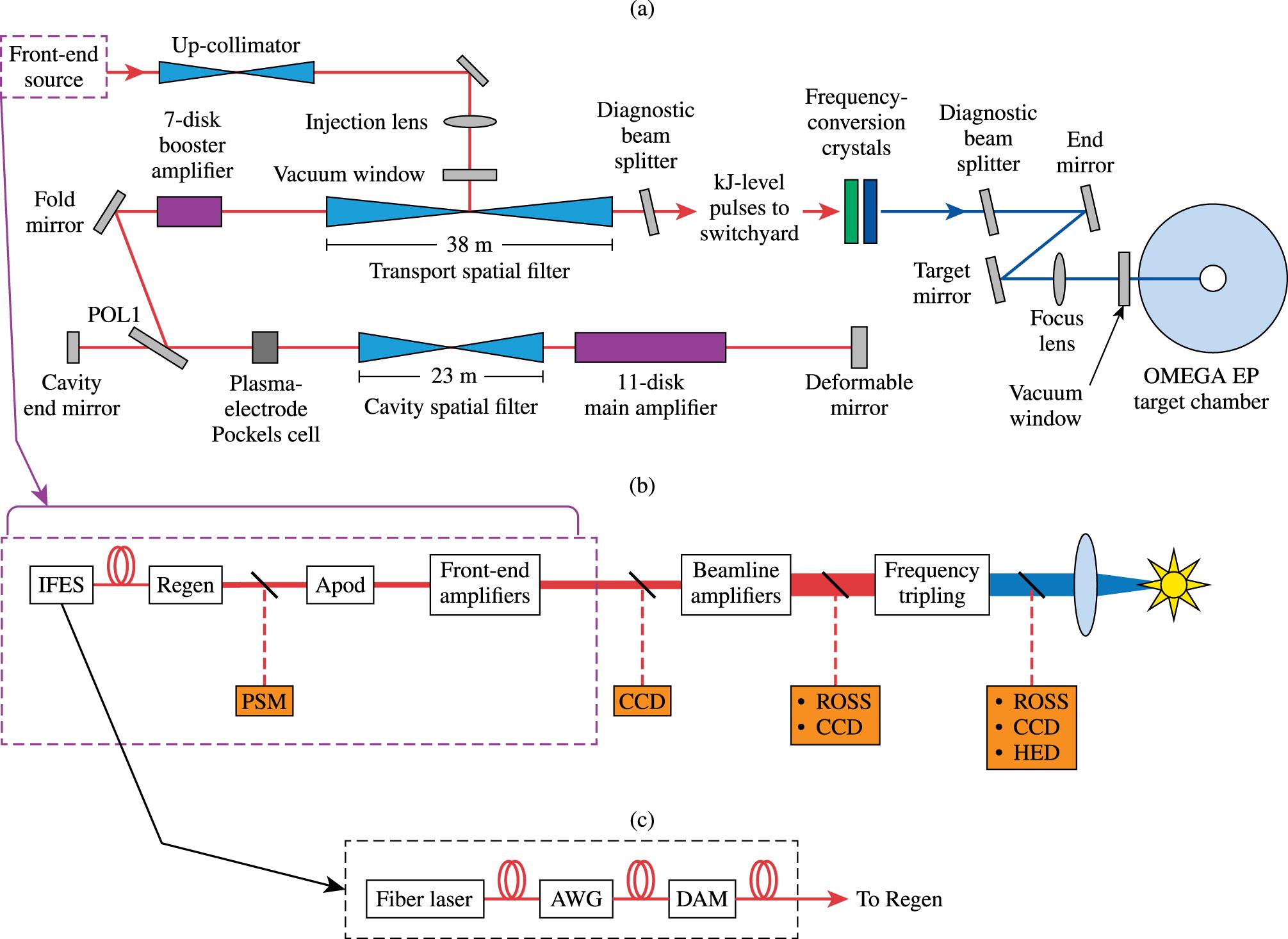
Fig. 1. OMEGA EP laser-system configuration. (a) Each of the four beamlines uses a folded architecture and type-I/type-II frequency-conversion crystal design based on the NIF. (b) Block diagram of (a) showing locations of pulse-shape, beam-profile and energy-measurement diagnostics used with the PSOPS model. PSM – pulse-shape monitor; Apod – beam-shaping apodizer; CCD – near-field camera; ROSS – Rochester optical streak system; HED – harmonic energy diagnostic. In addition to measuring near-field beam profile, CCD near-field cameras are calorimetrically calibrated to measure laser energy. (c) An integrated front-end system (IFES) produces temporally shaped 1053-nm seed pulses from a single-frequency, continuous-wave (cw) fiber laser. Precisely shaped temporal pulses are formed using an arbitrary waveform generator (AWG) that drives a dual-amplitude modulator.

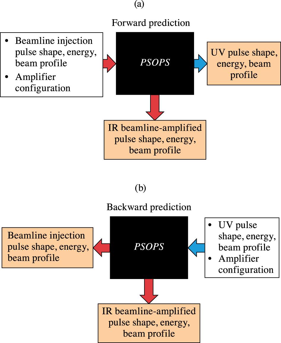
Fig. 2. Beamline pulse shape, energy and near-field beam profile are predicted in real time by PSOPS in forward and backward directions. (a) Forward prediction – UV beamline output is predicted using inputs to the amplifier chain and a specified amplifier configuration. (b) Backward prediction – IR stage energies, pulse shapes and near-field profiles are predicted using specified UV inputs and amplifier configuration.

Fig. 3. Plot of the inferred saturation fluence versus beamline output fluence from optimization fits to OMEGA EP beamline 3 data for nine-main-amplifier and seven-booster-amplifier configuration. Only shots with pulse widths and beam output energies ${\geqslant}2~\text{ns}$ and ${\geqslant}2~\text{kJ}$, respectively, were used in the fit.

Fig. 4. Pulse-width dependence of empirical scaling factor $[\unicode[STIX]{x1D6FE}(R)]^{-1}=[1+K\cdot B(R)]^{-1}$ to account for finite lifetime of the terminal laser level in Nd-doped phosphate laser glass, as per Ref. [41].

Fig. 5. (a) Fifteenth-order Legendre fit to the measured total small-signal gain for beamline 1, nine-main-amplifier configuration and (b) its $N\text{th}$ root (geometric mean) for the nine-disk, four-pass cavity where $N=36$. The single-disk small-signal gain shown in (b) is used in the PSOPS model when nine main amplifiers are configured for beamline 1.

Fig. 6. Horizontal lineouts of column-averaged, beamline 1 single-disk, small-signal gain maps for different numbers of main-amplifier disks fired. (a) Odd number of cavity amplifiers; (b) even number of cavity amplifiers.

Fig. 7. Flowchart illustrating the quasi-Newton method used for PSOPS forward predictions with a low-resolution grid. On the first iteration, the spatially-averaged output beam fluence $F_{\text{out}}$ is compared to $F_{\text{out}}$ from the calibration shot. The saturation fluence $F_{\text{sat}}$ is then scaled per the previously measured $F_{\text{sat}}$ vs. $F_{\text{out}}$ slope. Pulse-width correction to $F_{\text{sat}}$ is applied before the final (high resolution) simulation.

Fig. 8. Comparison of PSOPS forward-simulated amplified near-field beam profiles, pulse shapes and corresponding energies with measurements for beamline 3 shot 20,678. IR: 3112 J measured, 3102 J simulated. UV: 453 J measured, 452 J simulated. Simulations used measured injected beam profile, pulse shape and energy for shot 20,678.

Fig. 9. Comparison of PSOPS backward-simulated injected near-field beam profile, pulse shape and corresponding energy with measurements for beamline 3 shot 20,678: $79.5~\text{mJ}$ measured, $76.9~\text{mJ}$ simulated. Simulations used measured UV-beam profile, pulse shape and energy for shot 20,678.

Fig. 10. PSOPS forward-simulated UV pulses and UV ROSS measurements for beamline 1 shot 24,273. (a) The simulation used the directly measured injected pulse shape. (b) The measured injected pulse shape was first deconvolved using the estimated transfer function of the injected pulse measurement system. The transfer function was estimated using backward simulation from a different 100-ps pulse shot and improves the forward prediction of peak frequency-conversion efficiency. The measured full width at half maximum (FWHM) pulse width was 0.123 ns. Simulated FWHM pulse widths are given in the plots.

Fig. 11. (a) Predicted and requested UV pulse shapes showing how day-to-day changes in regen performance are compensated using PSOPS predictions; (b) post-shot UV pulse simulation, measurement and corresponding energies (beamline 3 shot 22,254). On-target UV energy: 775 J requested, 751 J measured, 752 J simulated.

Fig. 12. Examples showing facility flexibility enabled by PSOPS. (a) Based on an analysis of data from the previous shot, a significant increase in the slope of the UV pulse was desired while maintaining 220-J UV on-target energy. This request was accommodated by front-end pulse-shape and throttle adjustments prior to the next shot per the PSOPS pre-shot prediction. On-target UV energy: 220 J requested, 222 J measured (beamline 4 shot 20,647). (b) Different energies were requested while maintaining the original normalized design pulse shape that produced 500-J UV on-target energy. The measured UV on-target energies are shown in the label (beamline 3).

Fig. 13. (a) Pre-shot prediction and (b) measurement of approximately 27-ns composite UV pulse formed by incoherent addition of the individual beamline pulse shapes and beam-to-beam timing (shot 31,182).

Fig. 14. Measured beamline 3 output IR near-field beam-fluence profile (a) before moving the beam-shaping apodizer (contrast $=13.1\,\%$, peak to mean $=$ 1.46:1) and (b) after moving the apodizer by 0.49 mm (contrast = 9.4%, peak to mean $=$ 1.43:1). Contrast is defined in the text. The apodizer adjustment was guided by PSOPS simulations.

Fig. 15. Beamline 3 UV near-field beam-fluence profiles showing PSOPS-guided, multi-axis optimization of beam-shaping apodizer alignment to reduce the peak fluence in the amplified UV beam. A rotation of the apodizer by $3.5^{\circ }$, followed by lateral shifts of 0.36 mm (horizontal) and 0.24 mm (vertical) reduced the peak-to-mean UV-beam fluence. (a) Measured UV near-field beam before moving apodizer with peak-to-mean fluence of 3.74:1. (b) PSOPS simulation of (a). (c) PSOPS prediction after moving apodizer. (d) Measured UV beam after moving apodizer with peak-to-mean fluence of 2.76:1. The improved near-field profile shown in (d) was achieved using iterative PSOPS predictions followed by a single amplified UV shot.

Table 1. Comparison of PSOPS-simulations with measurements for SSG shots.