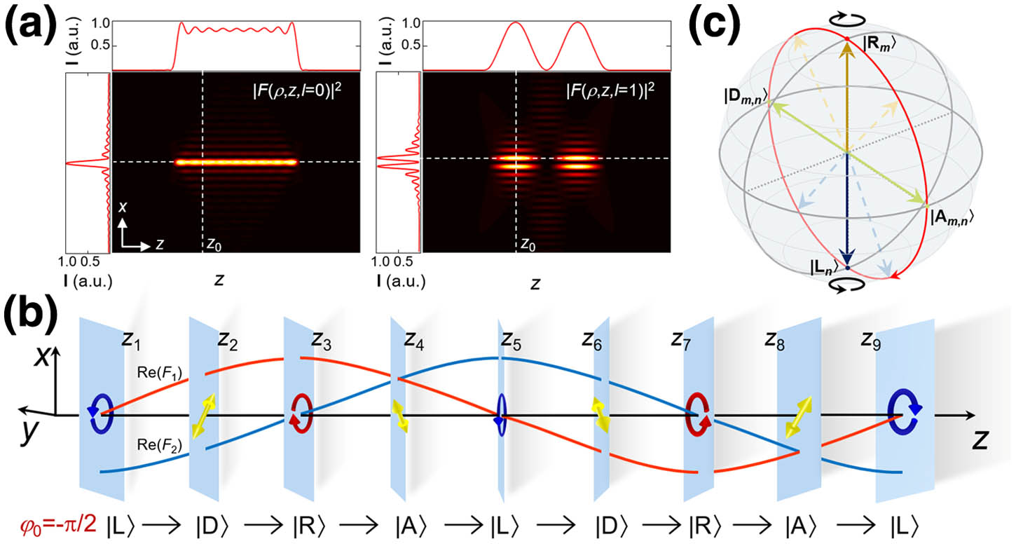
Fig. 1. Illustration of constructing polarization oscillating beams. (a) Zeroth- and first-order frozen waves that have rectangular and sinusoidal intensity profiles, respectively. The dashed lines denote where the intensity lines come from. (b) Evolution of transverse SoP of a polarization oscillating beam constructed from two sinusoidal frozen waves with opposite spin states and initial phase difference φ0=−π/2. The red and blue lines schematically depict the real parts of two electric fields. (c) Hybrid Poincaré sphere and the SoP conversion trajectory corresponding to the evolution in (b).

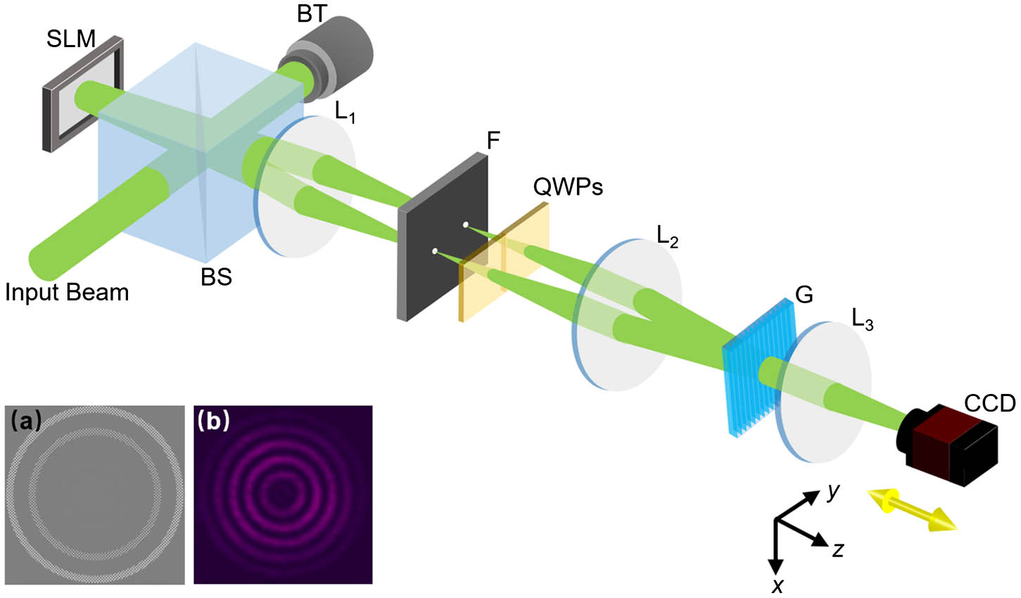
Fig. 2. Experiment setup for constructing polarization oscillating beams. SLM, spatial light modulator; BS, beam splitter; BT, beam terminal; L, lens; F, filter; QWP, quarter-wave plate; G, grating; CCD, charge-coupled device. Insets: (a) computer-generated hologram encoded on SLM; (b) intensity pattern of a first-order frozen wave at a certain location.

Fig. 3. Intensities of constituent zeroth-order frozen waves and transverse SoP distributions of the resultant field at different propagation distances, respectively. The red and cyan ellipses in the bottom diagrams denote the local polarization ellipticity calculated from the measured Stokes parameters [11].

Fig. 4. (a) Longitudinal intensity distributions of two first-order frozen waves (denoted as red dots and black squares) with sinusoidal profiles. Dots, experiment result; curves, analyzed results. (b) Lateral intensity patterns of the synthesized field in equally spaced planes.

Fig. 5. (a), (b) SoP distributions of the |D−1,1⟩ and |A−1,1⟩ states. (c)–(f) Experimentally measured SoP distributions at two adjacent nodes and antinodes. Left, polarization orientation (background) and polarization ellipticity distributions; right, S3 distributions. Black line and ellipse depict the linear and ellipse polarizations, respectively.

Fig. 6. (a) Intensity pattern of the second-order field at the z=0 plane. (b)–(e) Polarization orientation (upper) and intensity (bottom) distributions in four adjacent nodal planes. Arrows, the orientation of linear polarizer; dashed square, bound of selected areas corresponding to (b)–(e).

Fig. 7. (a) Intensity distribution of fifth-order field at the z=0 plane; (b)–(d) zoom-in vertical component distributions at three adjacent nodal planes.