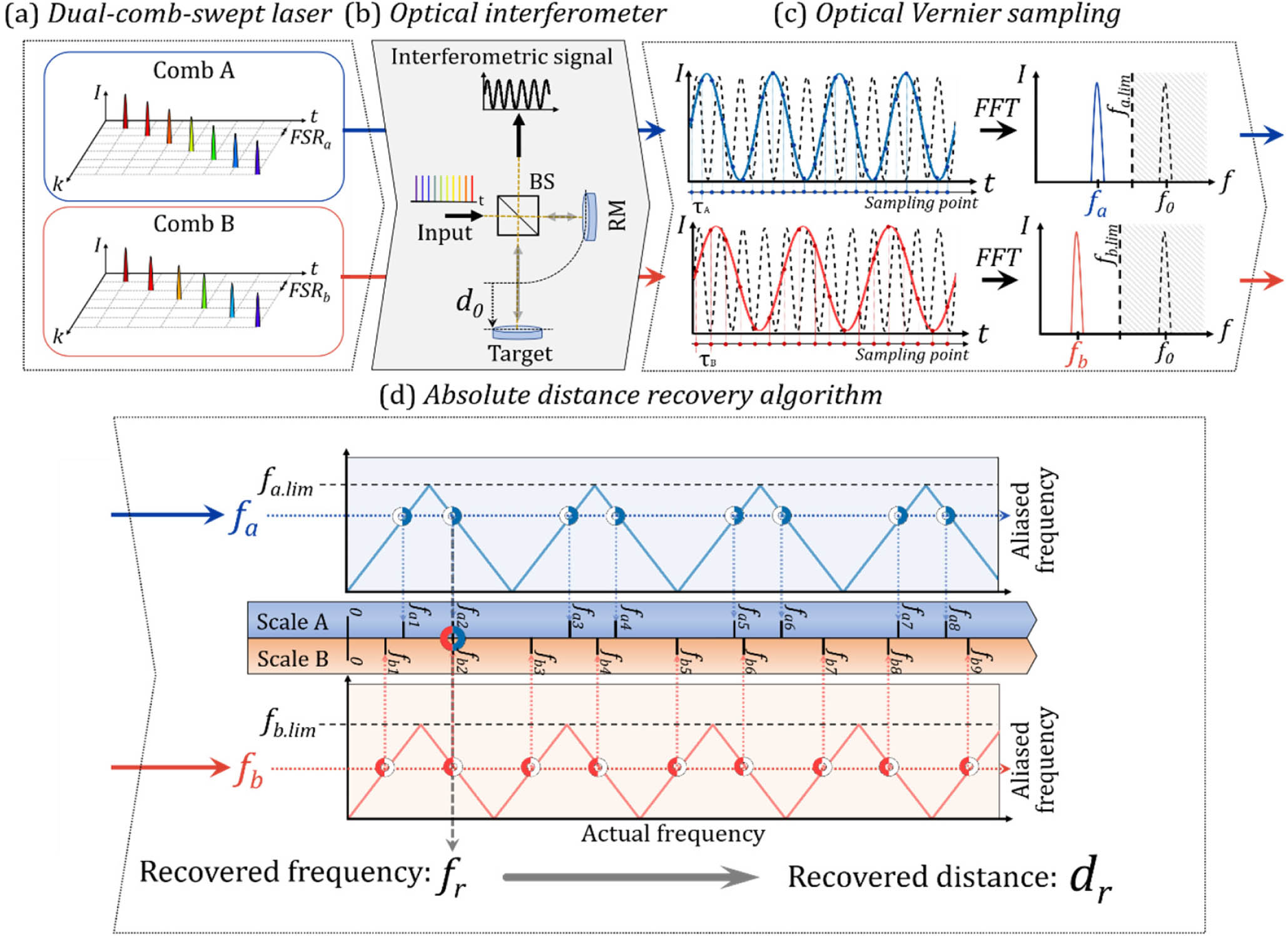
Fig. 1. Principle of the optical Vernier sampling method for solving distance aliasing. (a) A dual-comb-swept laser using comb A and comb B shows two different FSR values, namely, FSRa and FSRb, respectively. (b) Optical interferometer to measure the absolute distance of the target. BS, beam splitter; RM, reference mirror. (c) Actual interferometric signal using a continuous swept laser with a frequency of f0 (dashed line), and sampled interferometric signals using a proposed dual-comb-swept laser using comb A to indicate the aliasing frequency of fa (blue line) and using comb B to indicate the aliasing frequency of fb (red line), respectively. (d) Absolute distance recovery algorithm by measuring two aliasing frequencies of fa and fb together.

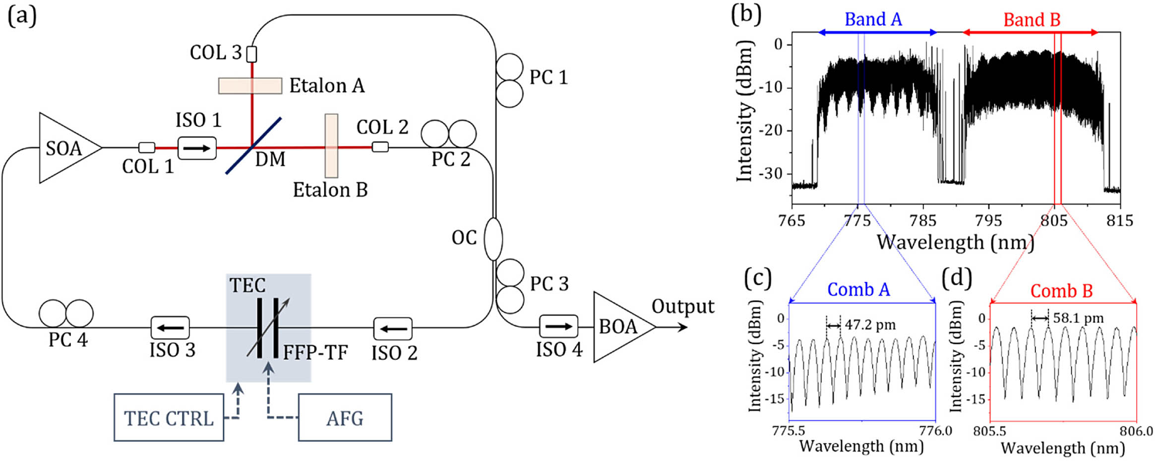
Fig. 2. (a) Setup of the dual-comb-swept laser. The black and red lines represent the fiber and free-space part, respectively. SOA, semiconductor optical amplifier; PC, polarization controller; COL, collimator; ISO, isolator; DM, dichroic mirror; OC, optical coupler; FFP-TF, fiber Fabry–Perot tunable filter; BOA, boosting optical amplifier; TEC, thermo-electric cooler; AFG, arbitrary function generator; TEC CTRL, TEC controller. (b) Optical spectrum of the peak hold mode obtained from the dual-comb-swept laser. Enlarged views of the spectra obtained using (c) comb A in the wavelength range of 775.5 to 776 nm and (d) comb B in the wavelength range of 805.5 to 806 nm.

Fig. 3. PSF measurements at every 0.4 mm interval using (a) comb A for the 1st and 12th orders and (c) comb B for the 1st and 11th orders. (b) and (d) show the collected first 0.4 mm positions of each forward aliased distance using combs A and B sources, respectively, for the 1st to 13th orders.

Fig. 4. Comparison of the recovered distance measurement with a numerical simulation.

Fig. 5. Multi-layer target measurement using a point-scanning setup. (a) Schematic of the point-scanning setup. OC, optical coupler; CIR, circulator; DL, delay line; BD, balanced detector. (b) Image of a multi-layer target. (c) Result of the multi-layer target measurement with refractive index compensation. (d) Cross-sectional view of the result at 15.68 mm along the Y axis (32nd pixel of the Y axis).

Fig. 6. 3D target measurement using a full-field imaging setup. (a) Schematic of the setup. L, lens; BS, beam splitter; RM, reference mirror. (b) Configuration of the 3D targets. Results showing the aliased distance using (c) comb A and (d) comb B sources. (e) Recovered distance data using combs A and B sources based on the optical Vernier sampling method.

Fig. 7. Recovered distance and SD obtained in the 3D target measurement using the full-field setup.

Fig. 8. Schematic showing the use of the recovery algorithm to obtain the recovered distance.

Fig. 9. Flowchart for the reference movement to solve the blind spot problem.

Fig. 10. Results of the numerical simulation employing the I/Q demodulation and frequency shifter.

Table 1. Result of Distance Measurement at Four Different Absolute Distances for 100 Times of Repetition (Unit: mm)