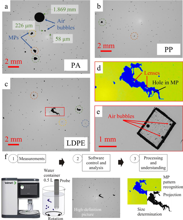
Fig. 1. Images acquired with Valmet FS5 UHD device for different samples in water including (a) PA particles, (b) PP particles, and (c) LDPE particles. (d) Zoomed-in and enhanced image of a microplastic particle from (c) (red contour). Red arrows in (d) highlight bright “lensing” areas in the microplastic particle. Black arrows in (d) highlights a hole in the MP. (e) Air bubbles on a PET MP. (f) Procedure to image and recognize MPs in a water sample.

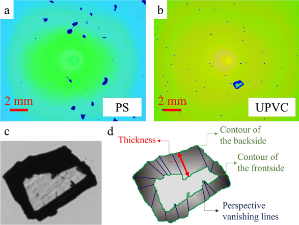
Fig. 2. Processed images in order to highlight the different plastic microparticles (a) PS and (b) UPVC plastic particles. Highlight on UPVC particle: (c) original cropped image and (d) contoured image showing an irregular-cut pyramid due to the grinding.

Fig. 3. Isolating MP from the acquired images and extracting an estimation of the projected surface area of the particle. (a) Original image, (b) cropped image, (c) isolated MP, and (d) projected image of the MP in black and white allowing an estimation of the size.

Fig. 4. Image of MP extracted from Figure 2c (LDPE samples) showing opening, facets, or “lenses” in the particles.

Fig. 5. Example of a 1 – M map obtained from one snapshot captured by UHD FS5 device. It shows a human hair, a kinked soft wood fiber, a PP microplastic and an air bubble. Each particle is further analyzed in Figure 6.

Fig. 6. Intensity distribution analysis through 1 – M values for (a) a human hair, (b) a soft wood fiber, (c) a microplastic, and (d) an air bubble. Left: 1 – M maps. Middle and right: cross-section along the colored arrows or dashed lines shown on the 1 – M maps. Insets in (c) and (d) are zoom-in curves on the central part of the 1 – M cross-sections.

Table 1. Selected MP extracted from Figure 1 to estimate the surface area: Plastic types and corresponding figures from which the MP images have been extracted; isolated MPs without background; projected images for pixels counting; surface area of the MP.