Linear and angular momenta in tightly focused vortex segmented beams of light (Invited Paper)

Martin Neugebauer; Andrea Aiello; Peter Banzer

doi:10.3788/COL201715.030003

Abstract

We investigate the linear momentum density of light, which can be decomposed into spin and orbital parts, in the complex three-dimensional field distributions of tightly focused vortex segmented beams. The chosen angular spectrum exhibits two spatially separated vortices of opposite charge and orthogonal circular polarization to generate phase vortices in a meridional plane of observation. In the vicinity of those vortices, regions of negative orbital linear momentum occur. Besides these phase vortices, the occurrence of transverse orbital angular momentum manifests in a vortex charge-dependent relative shift of the energy density and linear momentum density.

The linear and angular momenta (LM and AM) of light are of great importance in the description and understanding of dynamical processes concerning light-matter interaction phenomena. Representative examples are optical manipulation experiments, which demonstrate the possibility of transferring LM and AM from incoming light to trapped particles^[1–3]. For instance, spin AM results in a torque, while LM corresponds to a force or radiation pressure acting on a Rayleigh scatterer^[4,5]. A deep understanding of this type of light-matter interaction is particularly important in highly confined and/or structured electromagnetic fields^[6–8]. Recently, this led to a growing interest in the theoretical description^[5,9–11] and measurement^[12,13] of the individual constituents of LM and AM occurring in various nano-optical systems. In general, it is convenient to define these dynamical quantities locally, when complex three-dimensional field distributions are considered. Hence, we introduce the cycle-averaged LM density, $p = Re [E^{*} \times H] / c^{2}$ , which is proportional to the energy flow described by the Poynting vector, where the electric and magnetic fields $E$ and $H$ , respectively, are supposed to be monochromatic with an angular frequency $ω$ . The LM density can be separated into two distinct parts representing the spin ( $s$ ) and orbital ( $o$ ) contributions^[5–11], $p = p_{s} + p_{o} .$ (1)The spin LM density $p_{s}$ , sometimes referred to as Belinfante’s spin momentum density^[5,12–15], is defined by the curl of the spin AM density $s$ , $s = Im [ϵ_{0} E^{*} \times E + μ_{0} H^{*} \times H] / 4 ω,$ (2) $p_{s} = \nabla \times s / 2,$ (3)where $ϵ_{0}$ and $μ_{0}$ are the permittivity and permeability of the vacuum, respectively. In contrast, the orbital LM density is related to the phase gradients of all individual field components, weighted by their corresponding energy densities: $p_{o} = Im [ϵ_{0} E^{*} \cdot (\nabla) E + μ_{0} H^{*} \cdot (\nabla) H] / 4 ω .$ (4)Here, the notation $A \cdot (\nabla) B = A_{x} \nabla B_{x} + A_{y} \nabla B_{y} + A_{z} \nabla B_{z}$ is used. From Eqs. (2)–(4) it follows that both parts of the LM density can again be separated into electric and magnetic components^[9], with $p_{o} = p_{o E} + p_{o H}$ and $p_{s} = p_{s E} + p_{s H}$ .

In a simple single plane wave scenario, $p$ is by definition parallel to the propagation direction, while $s$ can be both, parallel, or antiparallel. In this case, since $s$ is independent of the position; it follows that $p_{s} = 0$ , and $p_{o} = p$ .

However, in highly confined field distributions more complex phenomena can occur. For example, regions of negative energy flow or regions where $p$ is antiparallel with respect to the global propagation direction of the light field occur in the waist of tightly focused beams^[16,17], in edge-diffracted fields^[18], and in the case of total internal reflection^[19–21]. Typically, these negative energy flows are linked to the occurrence of transverse vortices^[17–22]. Additionally, a negative longitudinal component of $p_{s}$ , which is linked to the occurrence of transverse components of $s$ , has been demonstrated in various optical systems consisting of propagating^[12,14] or evanescent waves^[5].

Sign up for Chinese Optics Letters TOC. Get the latest issue of Chinese Optics Letters delivered right to you！Sign up now

In this work, we investigate the occurrence of a negative longitudinal component of $p_{o}$ , a phenomenon sometimes referred to as ‘backflow’^[21,23–25], in tightly focused composite beams consisting of two spatially separated vortices with opposite charge and circular polarization of opposite handedness. Similar to a spin segmented beam^[26,27], focusing of such vortex segmented beams (VSBs) yields transverse AM, which depends on the charge of the input vortices^[28]. The transverse AM manifests itself in the occurrence of vortices oriented perpendicular to the propagation direction^{[17–22,29,30]}. Furthermore, it causes a relative shift of the centroids of the energy density and the LM density, which can be tuned by the vortex charge^[28]. We revisit this phenomenon for our VSB and highlight the different contributions of $p_{o}$ and $p_{s}$ .

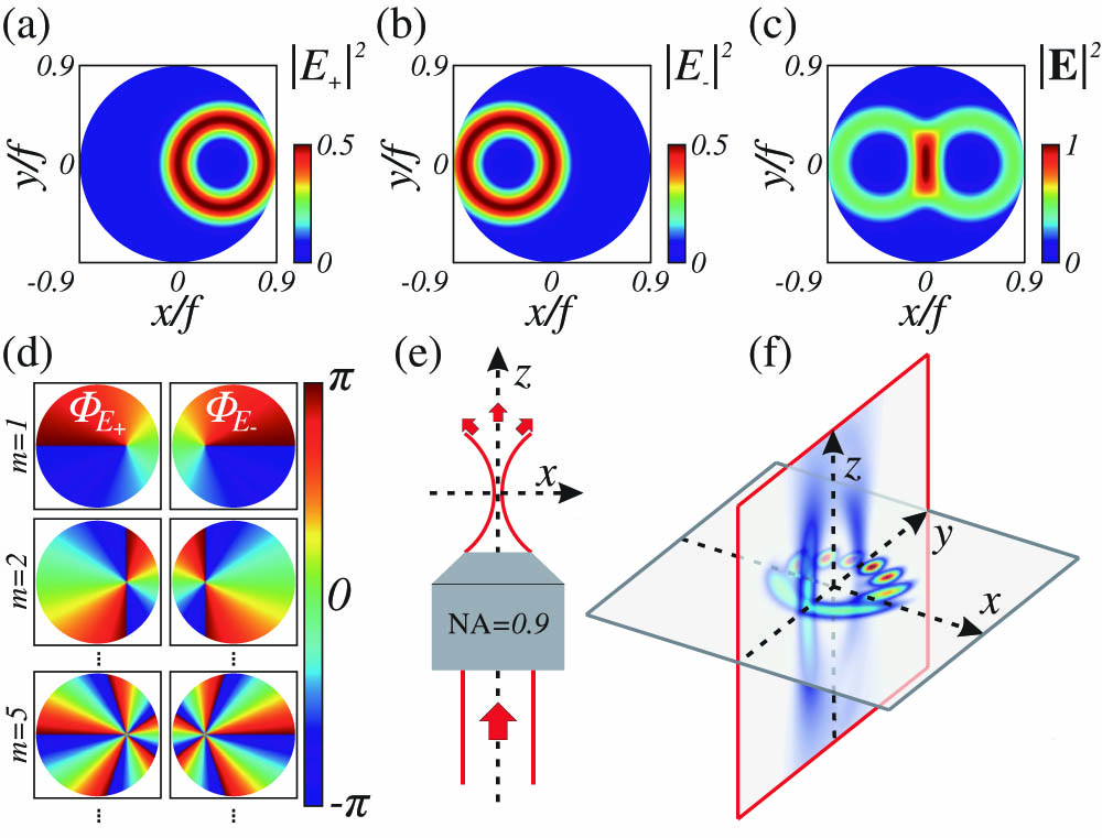
We begin by defining the input field distribution. It consists of two ringlike beams propagating along the $z$ axis and separated by a distance $2 d$ along the $x$ axis. The two beams have vortices with opposite charge $m$ and opposite handedness of the circular polarization ( $e_{\pm} = e_{x} \pm i e_{y}$ ): $E (x, y) = \exp [- {(\frac{a - \sqrt{{(x - d)}^{2} + y^{2}}}{w_{0}})}^{2}] \exp (i m φ_{+}) e_{+} + \exp [- {(\frac{a - \sqrt{{(x + d)}^{2} + y^{2}}}{w_{0}})}^{2}] \exp (i m φ_{-}) e_{-} .$ (5)Here, $\exp (i m φ_{\pm}) = {[(\pm x - d + i y) / {(x^{2} + y^{2})}^{1 / 2}]}^{m}$ , and $w_{0}$ determines the width of both beams. The radial distance between the maxima of the rings and their centroids is given by $a$ . As a focusing system, we consider an aplanatic microscope objective with a numerical aperture of $NA = R / f = 0.9$ , where $R$ is the aperture radius and $f$ is the focal length. Such objectives are commonly used in many microscopy setups. Here, we define $a = 0.4 f$ , $w_{0} = 0.2 f$ , $d = 0.4 f$ , and $m = 1$ to generate the field distribution in the back focal plane of the objective as depicted in Figs. 1(a)–1(c).

Figure 1.Input field distribution before focusing and planes of observation in the focal region. The field intensity distributions of the right- ( ${| E_{+} |}^{2}$ ) and left-handed ( ${| E_{-} |}^{2}$ ) circular polarization components in the aperture of the microscope objective are plotted in (a) and (b). The total electric field intensity ( ${| E |}^{2}$ ) is shown in (c). All three field intensity distributions are normalized to the maximum value of ${| E |}^{2}$ . (d) The phase distributions of the right- and left-handed fields ( $Φ_{E +}$ and $Φ_{E -}$ ) for different vortex charges $m$ . (e) The focusing scheme. (f) The focal $x - y$ plane is indicated by a gray frame, and the meridional $y - z$ plane is indicated by a red frame.

For higher-order vortex charges, only the phase distributions need to be adapted, as can be seen in Fig. 1(d). The focusing scheme, coordinate system, and the chosen orientation of the two different planes of observation that are used in the following discussions are depicted in Figs. 1(e) and 1(f). In the remainder, plots with a red frame indicate the meridional $y - z$ plane and images with a dark gray frame indicate the focal $x - y$ plane. Finally, we can start to discuss the focal field distributions that are calculated numerically with Richards–Wolf integrals^[16] following the formalism established in Ref. [31].

Figure 2 illustrates a side view of the tightly focused VSB with $m = 1$ . The total energy density distribution, $w = w_{E} + w_{H} = ε_{0} {| E |}^{2} / 4 + μ_{0} {| H |}^{2} / 4,$ (6)exhibits a ringlike shape in this meridional plane of observation [see Fig. 2(a)]. Considering the geometry of the beam, the $x$ component of the electric field is symmetric, whereas the $y$ and $z$ components are antisymmetric with respect to the $y - z$ plane.

Figure 2.Side view (meridional $y - z$ plane) of a VSB with charge number $m = 1$ in the focal region. (a) The total energy density distribution $w$ , (b) the energy density of the electric field $w_{E}$ , and (c) the energy density of the magnetic field $w_{H}$ are normalized to the maximum of $w$ . (d) The magnified phase distribution of the electric $x$ component $Φ_{E}^{x}$ . (e) The black arrowheads indicate the electric orbital LM density $p_{o E}$ in the vicinity of the vortex, with the distribution of $p_{o E}^{z}$ plotted in the background. The blue color indicates the unusual negative $p_{o E}^{z}$ , the red color indicates the positive $p_{o E}^{z}$ . The gray circles mark a vortex on the left side and a saddle point on the right side. (f) and (g) represent the electric spin LM density $p_{s E}$ and the total LM density $p \propto p_{o E} + p_{s E}$ , with the corresponding $z$ component plotted in the background. All three LM density distributions shown in (e)–(g) are normalized equally.

This implies that only the $x$ component of the electric field is present in this meridional plane of observation. For this reason, the distribution of the total energy density of the electric field ( $w_{E}$ ) depicted in Fig. 2(b) and the distribution of the $x$ component of the electric energy density ( $w_{E}^{x} = ε_{0} {| E_{x} |}^{2} / 4$ ) are the same in the shown plane. The magnetic energy density ( $w_{H}$ ) is shown in Fig. 2(c). Again, $w_{H}$ and $w_{E}$ exhibit ringlike distributions. For a further investigation of this structured field, we plot the phase distribution of the $x$ component of the electric field $Φ_{E}^{x}$ in Fig. 2(d). We see a typical phase vortex with charge one in the center of the ringlike distribution of $w_{E}^{x}$ [marked by a small black frame in Fig. 2(d)], however, this phase vortex occurs in a meridional plane and is therefore oriented transverse with respect to the global propagation direction^{[17–22,29,30,32]}. In order to examine this transverse vortex from a dynamical perspective, we illustrate the orbital LM $p_{o E}$ in the vicinity of the vortex in Fig. 2(e). On the left side, we observe a typical vortex structure that is accompanied by a saddle on the right side^[20,30,33]. Both structures are marked by gray circles. A similar distribution can also be found for $p_{o H}$ and $p_{o}$ (not shown here). In between the vortex and the saddle, the $z$ component of the electric orbital LM $p_{o E}^{z}$ exhibits negative values, which is emphasized by the color-coded distribution plotted in the background of Fig. 2(e). Blue and red indicate negative and positive $p_{o E}^{z}$ , respectively.

Such a negative $p_{o E}^{z}$ is particularly surprising, since all plane waves of the angular spectrum generating this field distribution exhibit a positive $p_{o E}^{z}$ . A small Rayleigh particle interacting only with the electric part of the field would therefore exhibit a radiation pressure force antiparallel to the overall LM of the light field, if it is located at such a position^[21]. In other words, the proposed beam would act like a ‘tractor beam’^[34], however, only in a very narrow range. For the sake of completeness, Figs. 2(f) and 2(g) additionally show the electric spin LM density $p_{s E}$ and the total LM density $p \propto p_{o E} + p_{s E}$ for the same plane of observation as in Fig. 2(e), respectively. Here, the spin LM shows a vortex with comparable strength, but opposite charge. Therefore, the total LM density is dominantly parallel to the $z$ axis. The major difference between the individual parts of the LM density highlights the importance of considering the constituents of $p$ separately.

In order to investigate the influence of the vortex charge of the incoming beam on the distributions of the energy densities and the LM densities, we exemplarily plot side view images similar to Figs. 2(a)–2(d) for a higher charge number of $m = 5$ in Figs. 3(a)–3(d). Again, we see a ringlike structure of $w$ , $w_{E}$ , $w_{E}^{x}$ , and $w_{H}$ , but the spatial extend of the distributions increased. Furthermore, instead of one vortex with charge 5 we now observe five single vortices with charge 1. This vortex splitting occurs^[29,35], since the aperture stop of the utilized focusing system causes clipping of the beam. Each vortex is accompanied by a saddle point and a region of negative $p_{o E}^{z}$ , similar to the vortex shown in Fig. 2. The number of vortices close to the focal point is determined by $m$ .

Figure 3.Side view of a VSB with charge number $m = 5$ in the focal region. The images in (a–d) are plotted similarly to Figs. 2(a)–2(d).

As a next step, we explore the distributions of the LM density and the energy density in the focal plane. Figure 4(a) shows the normalized distribution of $w$ in the focal plane, where the electric and magnetic $w_{E}$ and $w_{H}$ are plotted in the lower left and lower right insets.

Figure 4.Energy and LM in the focal plane. (a) and (b) depict the focal plane of a VSB with charge number $m = 1$ . (a) The energy densities $w$ , $w_{E}$ , and $w_{H}$ , are normalized to the maximum value of $w$ . (b) shows the corresponding LM components $p_{o}^{z}$ and $p^{z}$ , also normalized to the maximum value of $w$ . The other components $p^{x}$ , $p^{y}$ , $p_{o}^{x}$ , and $p_{o}^{y}$ are zero in the focal plane. The black scale bar represents the wavelength $λ$ . (c) and (d) show similar images plotted for a VSB with charge number $m = 5$ . (e) The $x$ positions of the centroids of $w$ (blue crosses), $p_{o}^{z}$ (red squares), and $p^{z}$ (black stars) are plotted against the charge index $m$ of the VSB.

Also in this plane of observation, $w$ exhibits a ringlike shape, however it is asymmetric with respect to the $x$ axis. Besides their interference pattern, $w_{E}$ and $w_{H}$ are unequally distributed in this regard. Actually, the centroids of all three distributions are shifted in the positive $y$ direction. In comparison, the centroids of the LM density distributions ( $p_{o}^{z}$ and $p^{z}$ ) are shifted in the negative $y$ direction [see Fig. 4(b)]. These shifts become even more recognizable when a higher charge is considered for the two incoming vortices. As an example, Figs. 4(c) and 4(d) show the focal energy density distributions and the focal LM density distributions for $m = 5$ . Clearly, the maxima and centroids of $w$ , $w_{E}$ , and $w_{H}$ are above the $x$ axis, whereas the maxima and the centroids of $p_{o}^{z}$ and $p^{z}$ are below the $x$ axis. To understand the reason for this striking difference between the energy density and the (orbital) LM density, we need to recall that $p_{o}^{z}$ is actually defined as the phase gradient of all individual field components, weighted by their corresponding energy densities. In the present scenario, the transverse LM components are exactly zero in the focal plane [see insets in Figs. 4(b) and 4(d)]. Therefore, any difference between the focal plane distributions of $p_{o}^{z}$ and $w$ must arise due to the phase gradient in the $z$ direction. Looking again at the phase distributions in Figs. 2(d) and 3(d), we recognize that the phase gradient to the left of the vortices is bigger than the phase gradient to the right. This notion directly links the relative shift between the LM densities and the energy densities to the occurrence of the phase vortices oriented transverse with respect to the propagation direction.

Finally, Fig. 4(e) depicts the $y$ coordinates of the centroids (all centroids lie on the $x$ axis) of the energy densities and the LM densities, plotted against the vortex charge of the respective incoming VSBs. Since the centroids of $w$ , $w_{E}$ , and $w_{H}$ as well as the centroids of $p_{o}^{z}$ , $p_{o E}^{z}$ , and $p_{o H}^{z}$ perfectly overlap, we consider only the centroids of $w$ ( $〈 y_{w} 〉$ ), $p_{o}^{z}$ ( $〈 y_{p o z} 〉$ ), and $p^{z}$ ( $〈 y_{p z} 〉$ ) in our discussion. All centroids depend linearly on the charge $m$ , with a positive slope for the energy density and negative slopes for the LM densities. The centroids $〈 y_{p o z} 〉$ and $〈 y_{p z} 〉$ always exhibit the same relative distance, independent of $m$ . Within the formalism developed in Ref. [36], we can associate this shift with the occurrence of transverse spin AM and the so-called geometric spin Hall effect of light^[27,28]. The relative shift between $〈 y_{p o z} 〉$ and $〈 y_{w} 〉$ can accordingly be attributed to the occurrence of transverse orbital AM and a geometric orbital Hall effect of light, since higher vortex charges yield bigger shifts^[28,37].

In conclusion, we investigate the focal region of tightly focused VSBs of light. The resulting transverse vortices indicate the generation of transverse orbital AM. In this regard, we also demonstrate the occurrence of negative orbital LM theoretically. A small Rayleigh scatterer would therefore feel a negative radiation pressure at such a position.

Furthermore, we discuss the relative shifts between the centroids of the energy density and the LM density, depending on the vortex charge of the incoming beam. A similar effect has already been reported for a slightly different focusing scenario in Ref. [28]. Here, we are able to link this relative shift to the occurrence of transverse vortices, in particular by exploring the orbital LM density in the focal region.

In general, the discussed field distributions with their focal points of zero field intensity and transverse AM might become relevant for stimulated emission depletion^[38] and optical manipulation experiments^{[1–4,13,34]}.

On the experimental side, such VSBs can be generated experimentally by utilizing spatial light modulators^[39] or Pancharatman–Berry phase optical elements^[40–42].

References

[1] A. Ashkin. Phys. Rev. Lett., 24, 156(1970).

[2] A. T. O’Neil, I. MacVicar, L. Allen, M. J. Padgett. Phys. Rev. Lett., 88, 53601(2002).

[3] V. Garcés-Chávez, D. McGloin, M. J. Padgett, W. Dultz, H. Schmitzer, K. Dholakia. Phys. Rev. Lett., 91, 93602(2003).

[4] M. Padgett, R. Bowman. Nat. Photonics, 5, 343(2011).

[5] K. Y. Bliokh, A. Y. Bekshaev, F. Nori. Nat. Commun., 5, 3300(2014).

[6] K. Y. Bliokh, F. Nori. Phys. Rep., 592, 1(2015).

[7] K. Y. Bliokh, F. J. Rodríguez-Fortuño, F. Nori, A. V. Zayats. Nat. Photonics, 9, 796(2015).

[8] A. Aiello, P. Banzer, M. Neugebauer, G. Leuchs. Nat. Photonics, 9, 789(2015).

[9] M. V. Berry. J. Opt. A, 11, 094001(2009).

[10] A. Aiello, P. Banzer. J. Opt., 18, 85605(2016).

[11] S. Saha, A. K. Singh, S. K. Ray, A. Banerjee, S. D. Gupta, N. Ghosh. Opt. Lett., 41, 4499(2016).