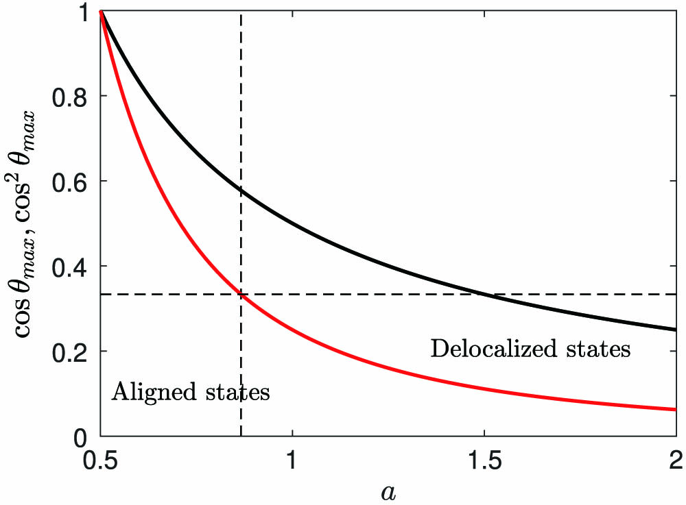
Fig. 1. Evolution of cos θ_max (black line) and cos²θ_max (red line) as a function of the parameter a. θ_max is the angle that maximizes the figure of merit F for a given value of a. The horizontal dashed line delimits the region of aligned and delocalized states. The area to the right of the vertical dashed line (of equation a=32) corresponds to simultaneous orientation and planar delocalization.

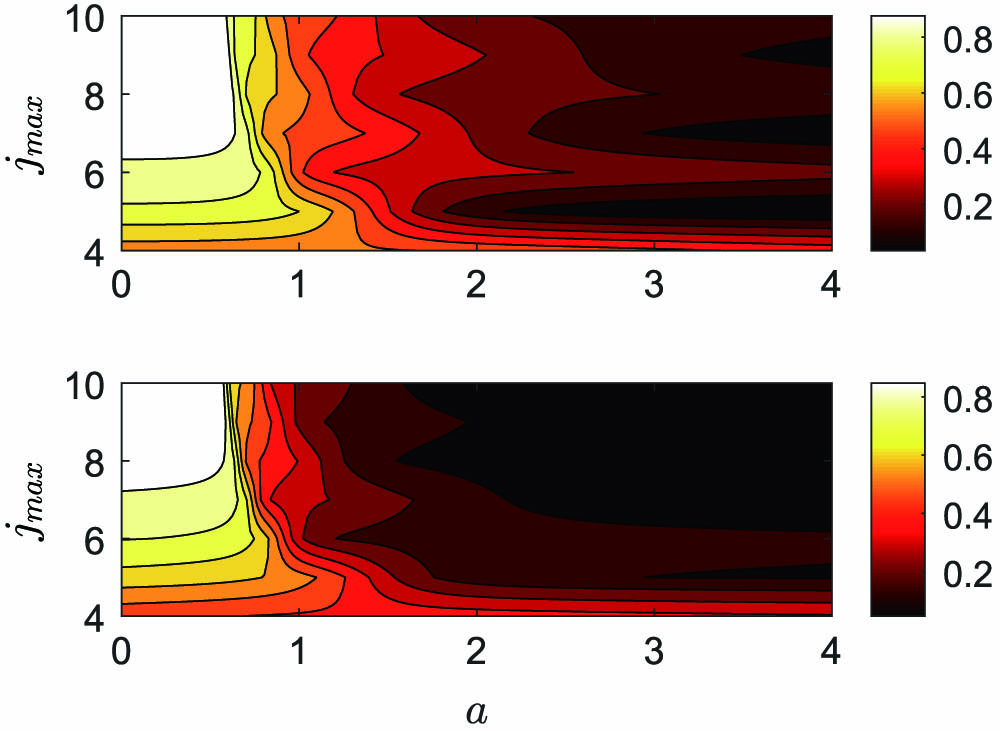
Fig. 2. Contour plot of the maximum of 〈cos θ〉 (top panel) and 〈cos²θ〉 (bottom panel) as a function of a and j_max.

Fig. 3. Probability density of the quantum state |ψ_T〉 maximizing the orientation and the planar delocalization simultaneously for a = 2 and j_max = 10.

Fig. 4. Evolution of the expectation values 〈cos θ〉 (black line) and 〈cos²θ〉 (red line) in the state |ψ_T〉 of a fictive molecule as a function of j_max for a = 2 (crosses). The solid lines are just to guide the reader. The horizontal dashed lines represent the classical values of cos θ and cos²θ for θmax=12a.

Fig. 5. Field-free time evolution of the expectation values 〈cos θ〉 (black line) and 〈cos²θ〉 (red line) of a fictive molecule at T = 0 K. The initial state at t = 0 is |ψ_T〉. The parameters a and j_max are set to 2 and 10. The horizontal dashed lines represent the classical values of cos θ and cos²θ for θmax=12a.

Fig. 6. (Top) Time evolution of 〈cos θ〉 (black line) and 〈cos²θ〉 (red line) for the CO molecule at T = 0 K under the action of the optimized pulse (bottom) followed by a field-free evolution of one rotational period. Numerical parameters are set to a = 2 and j_max = 10.

Fig. 7. Time evolution of 〈cos θ〉 (black line) and 〈cos²θ〉 (red line) for the CO molecule at T = 200 K [panel (a)] and 30 K [panel (b)] generated by a laser pulse followed by an HCP.

Fig. 8. Same as Fig. 7, but for the CH₃I molecule at T = 30 K. The HCP is replaced by a single-cycle pulse in the control process. Note that the range of time starts at time t/T_per = 0.25 in order to highlight the field-free evolution.