
Xiangda Lei, Hongtao Wang, Zongze Zhao. Small-Sample Airborne LiDAR Point Cloud Classification Based on Transfer Learning and Fully Convolutional Network[J]. Chinese Journal of Lasers, 2021, 48(16): 1610001
- Chinese Journal of Lasers
- Vol. 48, Issue 16, 1610001 (2021)

Fig. 1. Flow chart of the small sample point cloud classification based on transfer learning
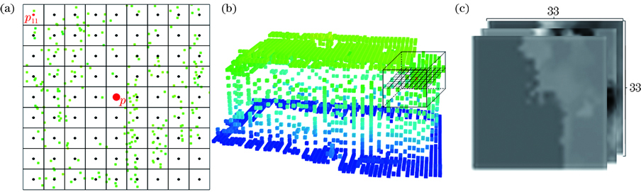
Fig. 2. Generation process of the point feature map. (a) Two-dimensional coordinates of the feature map; (b) point features in the cube neighborhood; (c) point feature map
Fig. 3. Generation of the multi-scale feature maps. (a) Grid size of 0.1 m; (b) grid size of 0.3 m; (c) grid size of 0.5 m
Fig. 4. Schematic diagram of the multi-projection. (a) X direction; (b) Y direction
Fig. 5. Deep feature extraction based on transfer learning
Fig. 6. Point cloud classification based on FCN
Fig. 7. Experimental datasets. (a) Training dataset displayed by normalized height; (b) aerial image corresponding to training dataset; (c) testing dataset displayed by normalized height; (d) aerial image corresponding to testing dataset
Fig. 8. F1 scores when classifying different feature combinations
Fig. 9. F1 scores when classifying different pre-training models
Fig. 10. Classification results when K=4
Fig. 11. Comparison of the misclassification results. (a) Misclassification result before graph-cuts optimization; (b) misclassification result after graph-cuts optimization
| ||||||||||||||||||||||||||||||||||||||||||||||||||||||||||||||||||||||||||||||||||||||||||||||||
Table 1. Influence of different K on the classification results unit: %
| |||||||||||||||||||||||||||||||||||||||||||||||||||||||||||||||||||||||||||||||||||||||||||||||||||||||||||||||||||||||
Table 2. F1 scores and overall classification accuracy of different methods unit: %
| |||||||||||||||||||||||||||||||||||||||||
Table 3. Classification results of our method and NANJ2 method unit: %
| ||||||||||||||||||||||||||||||||||||||||||||||||||||
Table 4. Classification results of different transfer learning methods unit: %

Set citation alerts for the article
Please enter your email address
© Copyright 2018-2021 | Chinese Laser Press. All Rights Reserved 沪ICP备15018463号-20