
Shijie Feng, Qian Chen, Guohua Gu, Tianyang Tao, Liang Zhang, Yan Hu, Wei Yin, Chao Zuo, "Fringe pattern analysis using deep learning," Adv. Photon. 1, 025001 (2019)
- Advanced Photonics
- Vol. 1, Issue 2, 025001 (2019)
Abstract
Optical measurement techniques such as holographic interferometry,1 electronic speckle pattern interferometry,2 and fringe projection profilometry3 are quite popular for noncontact measurements in many areas of science and engineering, and have been extensively applied for measuring various physical quantities, such as displacement, strain, surface profile, and refractive index. In all these techniques, the information about the measured physical quantity is stored in the phase of a two-dimensional fringe pattern. The accuracy of measurements carried out by these optical techniques is thus fundamentally dependent on the accuracy with which the underlying phase distribution of the recorded fringe patterns is demodulated.
Over the past few decades, tremendous efforts have been devoted to developing various techniques for fringe analysis. The techniques can be broadly classified into two categories: (1) phase-shifting (PS) methods that require multiple fringe patterns to extract phase information,4 and (2) spatial phase-demodulation methods that allow phase retrieval from a single fringe pattern, such as the Fourier transform (FT),5 windowed Fourier transform (WFT),6 and wavelet transform (WT) methods.7 Compared with spatial phase demodulation methods, multiple-shot PS techniques are generally more robust and can achieve pixel-wise phase measurement with higher resolution and accuracy. Furthermore, the PS measurements are quite insensitive to nonuniform background intensity and fringe modulation. Nevertheless, due to their multishot nature, these methods are difficult to apply to dynamic measurements and are more susceptible to external disturbance and vibration. Thus, for many applications, phase extraction from a single fringe pattern is desired, which falls under the purview of spatial fringe analysis. In contrast to PS techniques where the phase map is demodulated on a pixel-by-pixel basis, phase estimation at a pixel according to spatial methods is influenced by the pixel’s neighborhood, or even all pixels in the fringe pattern, which provides better tolerance to noise, yet at the expense of poor performance around discontinuities and isolated regions in the phase map.8,9
Deep learning is a powerful machine learning technique that employs artificial neural networks with multiple layers of increasingly richer functionality and has shown great success in numerous applications for which data are abundant.10,11 In this letter, we demonstrate experimentally for the first time, to our knowledge, that the use of a deep neural network can substantially enhance the accuracy of phase demodulation from a single fringe pattern. To be concrete, the networks are trained to predict several intermediate results that are useful for the calculation of the phase of an input fringe pattern. During the training of the networks, we capture PS fringe images of various scenes to generate the training data. The training label (ground truth) of each training datum is a pair of intermediate results calculated from the PS algorithm. After appropriate training, the neural network can blindly take only one input fringe pattern and output the corresponding estimates of these intermediate results with high fidelity. Finally, a high-accuracy phase map can be retrieved through the arctangent function with the intermediate results estimated through deep learning. Experimental results on fringe projection profilometry confirm that this deep-learning-based method is able to substantially improve the quality of the retrieved phase from only a single fringe pattern, compared to state-of-the-art methods.
Sign up for Advanced Photonics TOC. Get the latest issue of Advanced Photonics delivered right to you!Sign up now
Here, the network configuration is inspired by the basic process of most phase demodulation techniques, which is briefly recalled as follows. The mathematical form of a typical fringe pattern can be represented as
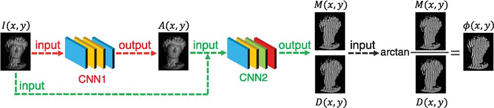
In order to emulate the process above, two different convolutional neural networks (CNN) are constructed, which are connected cascadedly according to Fig. 1. The first convolutional neural network (CNN1) uses the raw fringe pattern
![]()
Figure 1.Flowchart of the proposed method where two convolutional networks (CNN1 and CNN2) and the arctangent function are used together to determine the phase distribution. For CNN1 (in red), the input is the fringe image
To generate the ground truth data used as the label to train the two convolutional neural networks, the phase retrieval is achieved by using the
With the least square method, the phase can be calculated as
Thus, the numerator and the denominator of the arctangent function in Eq. (2) can be expressed as
The expressions above show that the numerator
To further reveal the internal structure of the two networks, the diagrams of the two convolutional neural networks are shown in Figs. 2 and 3. The labeled dimensions of the layers or the blocks show the size of their output data. The input of CNN1 is a raw fringe pattern with
![]()
Figure 2.Schematic of CNN1, which is composed of convolutional layers and several residual blocks.
![]()
Figure 3.Schematic of CNN2, which is more sophisticated than CNN1 and further includes two pooling layers, an upsampling layer, a concatenation block, and a linearly activated convolutional layer.
The performance of the proposed approach was demonstrated under the scenario of fringe projection profilometry. The experiment consisted of two steps: training and testing. In order to obtain the ground truth of training data, 12-step PS patterns with spatial frequency
To test the trained neural networks versus classic single-frame approaches (i.e., FT5 and WFT6), we measured a scene containing two isolated plaster models, as shown in Fig. 4(a). Compared with the right model, the left one has a more complex surface, e.g., the curly hair and the high-bridged nose. Note that this scenario was never seen by our neural networks during the training stage. The trained CNN1 using Fig. 4(a) as an input predicted a background intensity as shown in Fig. 4(b). From the enlarged views, we can see that the fringes have been removed completely through the deep neural network. Then, the trained CNN2 took the fringe pattern and the predicted background intensity as inputs and estimated the numerator
![]()
Figure 4.Testing using the trained networks on a scene that is not present in the training phase. (a) Input fringe image
Figures 5(a)–5(c) show the overall absolute phase errors of these approaches, and the calculated mean absolute error (MAE) of each method is listed in Table 1. Note that the adjustable parameters (e.g., the window size) in FT and WFT have been carefully tuned in order to get the best results possible. The result of FT shows the most prominent phase distortion as well as the largest MAE of 0.20 rad. WFT performed better than FT, with fewer errors for both models (MAE 0.19 rad). Among these approaches, the proposed deep-learning-based method demonstrates the least error, which is 0.087 rad. Furthermore, after the training stage, our method becomes fully automatic and does not require a manual parameter search to optimize its performance. To compare the error maps in detail, the phase errors of two complex areas are presented in Fig. 5(d): the hair of the left model and the skirt of the right one. From Fig. 5(d), obvious errors can be observed in the results of FT and WFT, which are mainly concentrated in the boundaries or abrupt depth-changing regions. By contrast, our approach greatly reduced the phase distortion, demonstrating its significantly improved performance in measuring objects with discontinuities and isolated complex surfaces. To further test and compare the performance of our technique with FT and WFT,
![]()
Figure 5.Comparison of the phase error of different methods: (a) FT, (b) WFT, (c) our method, and (d) magnified views of the phase error for two selected complex regions.
| Method | FT | WFT | Our |
| MAE (rad) | 0.20 | 0.19 | 0.087 |
Table 1. Phase error of FT, WFT, and our method.
For a more intuitive comparison, we converted the unwrapped phase into 3-D rendered geometries through stereo triangulation,13 as shown in Fig. 6. Figure 6(a) shows that the reconstructed result from FT features many grainy distortions, which are mainly due to the inevitable spectral leakage and overlapping in the frequency domain. Compared with FT, the WFT reconstructed the objects with more smooth surfaces but failed to preserve the surface details, e.g., the eyes of the left model and the wrinkles of the skirt of the right model, as can be seen in Fig. 6(b). Among these reconstructions, the deep-learning-based approach yielded the highest-quality 3-D reconstruction [Fig. 6(c)], which almost visually reproduced the ground truth data [Fig. 6(d)] where 12-step PS fringe patterns were used.
![]()
Figure 6.Comparison of the 3-D reconstruction results for different methods: (a) FT, (b) WFT, (c) our method, and (d) ground truth obtained by the 12-step PS profilometry.
It should be further mentioned that, in the above experiment, the carrier frequency of the fringe pattern is an essential factor affecting the performance of FT and WFT, which was set sufficiently high (
Finally, to quantitatively determine the accuracy of the learned phase after converting to the desired physical quantity, i.e., 3-D shape of the object, we measured a pair of standard ceramic spheres whose shapes have been calibrated based on a coordinate measurement machine. Figure 7(a) shows the tested ceramic spheres. Their radii are 25.398 and 25.403 mm, respectively, and their center-to-center distance is 100.069 mm. We calculated the 3-D point cloud from the phase obtained by the proposed method and then fitted the 3-D points into the sphere model. The reconstructed result is shown in Fig. 7(b), where the “jet” colormap is used to represent the data values of reconstruction errors. The radii of reconstructed spheres are 25.413 and 25.420 mm, with deviations of 15 and
![]()
Figure 7.Quantitative analysis of the reconstruction accuracy of the proposed method. (a) Measured objects: a pair of standard spheres and (b) 3-D reconstruction result showing the measurement accuracy.
In this letter, we have demonstrated how deep learning significantly improves the accuracy of phase demodulation from a single fringe pattern. Compared with existing single-frame approaches, this deep-learning-based technique provides a framework in fringe analysis by rapidly predicting the background image and estimating the numerator and the denominator for the arctangent function, resulting in high-accuracy edge-preserving phase reconstruction without any human intervention. The effectiveness of the proposed method has been verified using carrier fringe patterns under the scenario of fringe projection profilometry. We believe that, after appropriate training with different types of data, the proposed network framework or its derivation should also be applicable to other forms of fringe patterns (e.g., exponential phase fringe patterns or closed fringe patterns) and other phase measurement techniques for immensely promising applications.
Shijie Feng received his PhD in optical engineering at Nanjing University of Science and Technology. He is an associate professor at Nanjing University of Science and Technology. His research interests include phase measurement, high-speed 3D imaging, fringe projection, machine learning, and computer vision.
Qian Chen received his BS, MS, and PhD degrees from the School of Electronic and Optical Engineering, Nanjing University of Science and Technology. He is currently a professor and a vice principal of Nanjing University of Science and Technology. He has been selected as Changjiang Scholar Distinguished Professor. He has broad research interests around photoelectric imaging and information processing, and has authored more than 200 journal papers. His research team develops novel technologies and systems for mid-/far-wavelength infrared thermal imaging, ultrahigh sensitivity low-light-level imaging, noninterferometic quantitative phase imaging, and high-speed 3D sensing and imaging, with particular applications in national defense, industry, and bio-medicine. He is a member of SPIE and OSA.
Guohua Gu received his BS, MS, and PhD degrees at Nanjing University of Science and Technology. He is a professor at Nanjing University of Science and Technology. His research interests include optical 3D measurement, fringe projection, infrared imaging, and ghost imaging.
Tianyang Tao received his BS degree at Nanjing University of Science and Technology. He is a fourth-year PhD student at Nanjing University of Science and Technology. His research interests include multiview optical 3D imaging, computer vision, and real-time 3D measurement.
Liang Zhang received his BS and MS degrees at Nanjing University of Science and Technology. He is a fourth-year PhD student at Nanjing University of Science and Technology. His research interests include high-dynamic-range 3D imaging and computer vision.
Yan Hu received his BS degree at Wuhan University of Technology. He is a fourth-year PhD student at Nanjing University of Science and Technology. His research interests include microscopic imaging, 3D imaging, and system calibration.
Wei Yin is a second-year PhD student at Nanjing University of Science and Technology. His research interests include deep learning, high-speed 3D imaging, fringe projection, and computational imaging.
Chao Zuo received his BS and PhD degrees from Nanjing University of Science and Technology (NJUST) in 2009 and 2014, respectively. He was a research assistant at Centre for Optical and Laser Engineering, Nanyang Technological University from 2012 to 2013. He is now a professor at the Department of Electronic and Optical Engineering and the principal investigator of the Smart Computational Imaging Laboratory (www.scilaboratory.com), NJUST. He has broad research interests around computational imaging and high-speed 3D sensing, and has authored over 100 peer-reviewed journal publications. He has been selected into the Natural Science Foundation of China (NSFC) for Excellent Young Scholars and the Outstanding Youth Foundation of Jiangsu Province, China. He is a member of SPIE, OSA, and IEEE.
References
[1] T. Kreis. Handbook of Holographic Interferometry: Optical and Digital Methods(2006).
[2] P. K. Rastogi. Digital Speckle Pattern Interferometry & Related Techniques(2000).


Set citation alerts for the article
Please enter your email address

© Copyright 2018-2021 | Chinese Laser Press. All Rights Reserved 沪ICP备15018463号-20