• Photonics Research
  • Vol. 11, Issue 3, 442 (2023)
Yao Fan1、2、3, Jiasong Sun1、2、3, Yefeng Shu1、2、3, Zeyu Zhang1、2、3, Qian Chen1、2、3、4、*, and Chao Zuo1、2、3、5、*
Author Affiliations
  • 1Smart Computational Imaging (SCI) Laboratory, Nanjing University of Science and Technology, Nanjing 210094, China
  • 2Smart Computational Imaging Research Institute (SCIRI) of Nanjing University of Science and Technology, Nanjing 210019, China
  • 3Jiangsu Key Laboratory of Spectral Imaging & Intelligent Sense, Nanjing University of Science and Technology, Nanjing 210094, China
  • 4e-mail: chenqian@njust.edu.cn
  • 5e-mail: zuochao@njust.edu.cn
  • show less
    DOI: 10.1364/PRJ.476170 Cite this Article Set citation alerts
    Yao Fan, Jiasong Sun, Yefeng Shu, Zeyu Zhang, Qian Chen, Chao Zuo. Accurate quantitative phase imaging by differential phase contrast with partially coherent illumination: beyond weak object approximation[J]. Photonics Research, 2023, 11(3): 442 Copy Citation Text show less

    Abstract

    Quantitative phase imaging (QPI) by differential phase contrast (DPC) with partially coherent illumination provides speckle-free imaging and lateral resolution beyond the coherent diffraction limit, demonstrating great potential in biomedical imaging applications. Generally, DPC employs weak object approximation to linearize the phase-to-intensity image formation, simplifying the solution to the phase retrieval as a two-dimensional deconvolution with the corresponding phase transfer function. Despite its widespread adoption, weak object approximation still lacks a precise and clear definition, suggesting that the accuracy of the QPI results, especially for samples with large phase values, is yet to be verified. In this paper, we analyze the weak object approximation condition quantitatively and explicitly give its strict definition that is applicable to arbitrary samples and illumination apertures. Furthermore, an iterative deconvolution QPI technique based on pseudo-weak object approximation is proposed to overcome the difficulty of applying DPC to large-phase samples without additional data acquisition. Experiments with standard microlens arrays and MCF-7 cells demonstrated that the proposed method can effectively extend DPC beyond weak object approximation to high-precision three-dimensional morphological characterization of large-phase technical and biological samples.

    1. INTRODUCTION

    Phase contrast imaging is an essential label-free imaging technique because it enables the visualization of biological processes at multiple scales and resolutions in a non-invasive manner, providing a unique tool for cell division [1], intracellular dynamics [2], phenotypic screening [3], etc. It manipulates scattered radiation through optical field modulations to convert the phase information of non-self-luminous and non-absorbing samples into intensity signals. One of the most classical phase contrast imaging methods is based on interferometric imaging [usually quantitative, also known as quantitative phase imaging (QPI)] [47], whose highest spatial frequency, however, is confined to coherent diffraction limit NAλ, leading to a limited lateral resolution and poor environmental stability.

    Partially coherent illumination endows phase contrast imaging with the superiority of high robustness and significantly extended lateral resolution, prompting its applications in biological imaging. The pioneering techniques in this field, such as Zernike phase contrast and differential interference contrast (DIC), have become standard solutions for cellular and subcellular observation [812]. Recent advances in partially coherent imaging have further boosted to the development of a series of QPI techniques, such as transport-of-intensity equation (TIE) [1315], differential phase contrast (DPC) [1618], and Fourier ptychographic microscopy (FPM) [1924]. These techniques quantify the optical path length fluctuations across transparent samples and acquire three-dimensional (3D) quantitative phase, enabling phase contrast imaging to move from “qualitative” to “quantitative” [15,2528]. Because of their superior imaging performance and flexible experimental configuration, QPI techniques have demonstrated their great potential in diverse biological applications [2932].

    QPI by DPC with partially coherent imaging is realized through asymmetric illumination modulation and deconvolution reconstruction, providing speckle-free imaging and twice the lateral resolution of the coherent diffraction limit [33,34]. It estimates the quantitative phase distribution of the sample from the measured intensities, which is considered to solve an inverse problem [35,36]. A strict and correct “intensity-phase” model is required to achieve accurate phase retrieval. However, mutual incoherence of the illumination points results in the nonlinear (or, more precisely, bilinear) dependence of the partially coherent field on the sample properties, which makes it a daunting challenge to recover the sample phase through intensity inversion. Thus, the primary task of QPI with partially coherent imaging is to accurately explain the nonlinear (bilinear) image generation model, a fundamental issue of great importance for the development of QPI. A well-established model is based on the transmission cross-coefficient (TCC) model, which establishes a four-dimensional (4D) expression on the pairs of spatial frequencies of the sample in the spatial frequency domain [37,38] so that the contribution of the sample- and system-dependent parts are represented separately. In addition, the phase-space representations, expressed through 4D Winger functions in the joint spatial frequency domain, model its bilinear characteristics with the advantage of separating the imaging system and the sample [3942]. However, these high-dimensional representations are difficult to obtain precisely, while their massive data and computation costs make it impractical to recover sample information.

    The preferred solution to achieve QPI under partially coherent imaging is to simplify the bilinear transmission of image information as linear properties. For this purpose, the sample (or object) approximations, including weak/slowly varying object approximation [17,33], Born/Rytov approximation [43,44], and multi-slice scattering approximation [45], have been proposed, all of which brought new insights into QPI. For example, weak object approximation considers the amplitude of the scattered light is much smaller than that of the unscattered light, linearizing the relationship between recorded intensity and sample transmission [46,47]. Then, a regularization deconvolution solver is proposed to recover the quantitative phase of the sample [17,48]. Slowly varying object approximation establishes a phase-gradient sensitive mechanism, leading to a “lookup table” correspondence between the measured intensity and the sample phase gradient [49,50]. However, the introduction of approximations means that the imaging performance of the algorithms derived from them is limited by how well the real sample matches the approximation model, making accurate phase (thickness) reconstruction of diverse samples from QPI alone difficult. Moreover, the explicit definitions of these approximations in existing work are still poorly understood. These limitations may result in QPI losing its proudest “quantitative” properties and no longer providing credible evidence for subsequent analyses such as cell morphology and cell mass measurement [51,52].

    In this paper, we explore the strict definition of weak object approximation and further propose an iterative deconvolution DPC QPI technique that achieves accurate quantitative phase reconstruction without any additional acquisition, allowing QPI to be extended for biology applications of large-phase samples. The strict definition of weak object approximation is explicitly stated: the one-step deconvolution method could obtain accurate quantitative phase results only when the sample phase is not greater than 0.5 rad. Furthermore, to overcome the difficulty of applying DPC to large-phase samples, we introduce a pseudo-weak object approximation to model the complex transmittance function of the sample and propose an iterative deconvolution algorithm to achieve accurate QPI without additional data acquisition. The iterative process is performed with a deconvolution solver to refine the phase; thus, the phase components can be fully decoupled from the acquisition intensity. We conduct an experiment using a standard microlens array with a large phase of 37 rad (23 μm) and verify that the proposed method yields a quantitative phase consistent with the nominal value. Furthermore, the experiment results on MCF-7 cells accurately present the 3D morphological distribution of the cells, which demonstrates great potential for cell morphology and cell mass measurements.

    2. STRICT WEAK OBJECT APPROXIMATION CONDITION

    A. Quantitative Phase Imaging by DPC Based on Weak Object Approximation

    QPI based on partially coherent imaging provides better lateral resolution and immunity to the system’s imperfections by simultaneously illuminating the sample from multiple angles in a mutually incoherent manner. The light intensity follows Abbe diffraction theory [53], i.e., mutual incoherence of the illumination points leads to the incoherent superposition of the intensity caused by each point. The cross propagation and superposition of each point often result in the nonlinear (or, more precisely, bilinear) dependence of the partially coherent field on the sample properties [37,38,54]: I(x)=S(u)T(u1)T*(u2)H(u+u1)H*(u+u2)ej2πx·(u1u2)du1du2du,where x represents the two-dimensional (2D) coordinates of the camera plane, and u represents the spectrum coordinates. The sample is represented as a Fourier spectrum form of its complex transmittance function T(u)=F{ejϕ(x)} [where ϕ(x) is the phase of the sample], and T(u1)T*(u2) is its mutual spectrum. S(u) represents the partially coherent illumination source, which is usually an extended source whose illumination NA is less than or equal to the NA of the objective lens. H(u) represents the coherent transfer function (CTF), which can be expressed as H(u)=P(u)ejkδz1(λux)2(λuy)2 [P(u) is the pupil function of the objective lens, and ejkδz1(λux)2(λuy)2 is the defocusing factor for propagating the light field on different planes]. From Eq. (1), the intensity I(x) of each point in the image is considered as a point pair dependent on the sample amplitude. To separate the effects of the system and the sample properties, the sample-independent factors are established as TCC (or the partially CTF in Sheppard’s paper Ref. [33]), which is a 4D function of pairs of spatial frequencies: TCC(u1,u2)=S(u)H(u+u1)H*(u+u2)du.

    This equation illustrates that TCC is determined by the illumination function S(u) and CTF, and it establishes a quantitative relationship between sample distribution and acquired intensity. It can be found from Eq. (1) that the contributions from sample amplitude and phase in the intensity signal under partially coherent imaging cannot be expressed explicitly. This makes it a daunting challenge to recover the sample phase through intensity inversion.

    Object approximation is the most common method for simplifying the partially coherent imaging model to a mathematically analytic form [34]. Weak object approximation achieves the linearization of the intensity expression, establishing an effective phase inversion mechanism (the forward model of partially coherent imaging and QPI algorithm are given in Appendices A and B). It requires the phase terms of the sample to be very weak (usually much less than 1 rad), and then the complex transmittance function of the sample t(x)=ejϕ(x) can be approximated as t(x)=ejϕ(x)1+jϕ(x).

    This expression ignores a series of higher-order terms in phase and retains only its primary term, successfully separating the DC (background) and phase terms into the real and imaginary parts of the complex distribution. Then, a linear expression of mutual intensity is substituted into Eq. (1) to obtain the intensity distribution under the weak phase approximation [55], I(x)TCC(0,0)+2Re{TCC(u,0)[jΦ(u)]ej2πx·udu},where TCC(0,0) is the direct current (DC) component (the background). TCC(u,0) is the weak phase transfer function (WPTF), characterizing the quantitative relationship between the sample phase and the acquisition intensity. For QPI, which converts jΦ(u) to the intensity with real distribution modulated by WPTF, the illumination S(u) or CTF H(u) modulations are required to produce a phase transfer response with an oddly symmetric distribution.

    DPC adopts asymmetric illumination, a flexible and convenient implementation without mechanical manipulation, to achieve an oddly symmetric WPTF and evenly symmetric absorption transfer function [16,17]. Consequently, a simple differential calculation can be implemented to eliminate the background item from Eq. (4), and only linear phase items are left in IiDPC(x), IiDPC(x)=Ii1(x)Ii2(x)Ii1(x)+Ii2(x),where i indicates the direction of asymmetric illumination Si(u), and Ii1(x) and Ii2(x) denote the two intensity images along the same asymmetric axis. Then, the corresponding WPTF can be expressed as WPTF(u)=Si(u)H*(u+u)H(u)Si(u)H(uu)H*(u)du|Si(u)||H(u)|2du.

    This leads to a linear relationship between the phase of the sample and the acquired intensity, and the quantitative phase information can then be reconstructed by Fourier space deconvolution with the WPTF [1618,56]. Tikhonov regularization is commonly used to solve the ill-posed problem to obtain a stable approximate solution, ϕ(x)=F1{i[WPTFi*(u)·IiDPC(u)]i|WPTFi(u)|2+β},where β represents the regularization parameter to avoid excessive amplification of noise.

    B. Illumination and Nonlinear Error of Weak Object Approximation

    Weak object approximation simplifies partially coherent imaging; however, it also limits the applicability of the phase inversion algorithm. Specifically, only if the weak object condition is met can the quantitative phase distribution of the sample be recovered accurately without distortions and artifacts. Otherwise, DPC will suffer from severe nonlinear errors and lose its nature of “quantitative.” The analysis of the theoretical model of the deconvolution solution reveals that two approximations are involved in its derivation. On the one hand, weak object approximation linearizes the complex transmittance function of the sample by omitting the higher-order terms in its Taylor expanded form, as shown in Eq. (3). On the other hand, the higher-order scattering terms are ignored to derive the analytical expression of the WPTF, as shown in Eq. (4). Although the two approximations jointly contribute to the deconvolution reconstruction algorithm, the intensity difference of Eq. (5) eliminates the nonlinear error caused by the latter approximation. Thus, the reconstruction error in the DPC deconvolution mainly arises from the mismatch between the ideal sample function ejϕ(x) and the linear sample function 1+jϕ(x). In Appendix C, we prove this conclusion by simulating the one-step deconvolution reconstruction under both sample models, and the results are shown in Fig. 7. In addition, a critical corollary suggests that although weak object approximation is only described as a sample simplification model (which appears to be relevant only to the sample’s absolute phase), the acquired intensity under angularly varying illumination exhibits different nonlinear characteristics. Then, weak object approximation will result in different degrees of information being ignored. This implies that the mismatch between the actual and linear intensity model under weak object approximation is related to illumination aperture.

    Figure 1 explains the information mismatch between the actual and linear intensity model under weak object approximation with different illumination by numerical simulation. The complex transmittance functions of ejϕ(x) and 1+jϕ(x), which express the actual sample distribution and the linear distribution, were used to generate the DPC acquisition images at different illumination coefficients sill (where sill=NAillNAobj, indicating the ratio of illumination NAill and objective NAobj). The acquisition images were defined on a grid with 400×400  pixels with a pixel size of 0.3  μm×0.3  μm. The wavelength of the illumination is 525 nm, and the NAobj is 0.4. All subsequent simulations follow these parameter configurations. The corresponding intensity differences and root mean square error (RMSE) values were then calculated to measure the model mismatch, as shown in Figs. 1(d) and 1(e). It can be seen that the intensity difference between the two sample models grows exponentially with the increasing illumination coherence coefficients (sill from 0 to 1). This will result in inaccurate phase reconstruction by the deconvolution solver under weak object approximation. We further display the reconstructed phase at sill=1 in Fig. 1(e), which shows a significantly weaker phase value compared to the ground-truth phase. Figure 1(f) shows the 3D morphological distribution of the phase loss of the reconstructed phase compared to the ground-truth phase. In Appendix C (Figs. 7 and 8), two simulations further illustrate that the imaging performance of the one-step deconvolution solver is related to the illumination aperture. Therefore, a conclusion can be drawn that the definition of weak object approximation should not only consider the sample but should be analyzed in terms of the QPI performance to take into account the illumination aperture and sample.

    Simulation and comparison of ideal intensity model and weak object approximation intensity model under different illumination coefficients. (a) Ground-truth amplitude and phase images of the complex transmittance function used to simulate the sample. (b) Spectrum distribution of the theoretical sample distribution ejϕ(x) and linear distribution 1+jϕ(x). (c) Different illumination coefficients. (d) Intensity difference images at different illumination coefficients sill. (e) RMSE values of the intensities under two sample models with varying illumination coefficients. (f) 3D profile of the reconstructed phase error at sill=1.

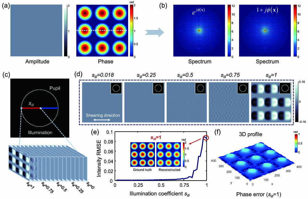
    Figure 1.Simulation and comparison of ideal intensity model and weak object approximation intensity model under different illumination coefficients. (a) Ground-truth amplitude and phase images of the complex transmittance function used to simulate the sample. (b) Spectrum distribution of the theoretical sample distribution ejϕ(x) and linear distribution 1+jϕ(x). (c) Different illumination coefficients. (d) Intensity difference images at different illumination coefficients sill. (e) RMSE values of the intensities under two sample models with varying illumination coefficients. (f) 3D profile of the reconstructed phase error at sill=1.

    C. Strict Weak Object Approximation Condition

    The well-defined weak object approximation is the basis for guaranteeing the accuracy of quantitative phase reconstruction, while it also allows the imaging performance of QPI to be measured and analyzed in an informed manner. However, due to the complex theoretical derivation of the deconvolution solver, it is challenging to determine the strict definition of weak object approximation from the mathematical expression. To address this problem, we analyzed the imaging performance of DPC QPI at maximum nonlinear error to explore the strict weak object approximation definition applicable to all samples and illumination apertures. Two representative samples of a slowly varying microlens array and three sharply varying steps were selected as target samples, and their phase amplitudes can be adjusted arbitrarily. Meanwhile, the illumination aperture can be set from half-circle to half-annulus to simulate different illuminations. The largest nonlinear error will arise when the sample of three sharply varying steps is illuminated by a half-annular aperture with the maximum illumination coefficient. In this case, an accurate reconstruction of the sample phase using the one-step deconvolution will serve as the basis for the strict definition of weak object approximation.

    Figure 2 shows the numerical simulation results for two representative samples with varying phases from 0.2 rad to 2 rad under different illumination apertures. As shown in Fig. 2(a), three types of illumination apertures were set, including a half-circular aperture, a half-annular aperture of 0.5 width, and a half-annular illumination of 0.01 width with the maximum illumination coefficient. The half-circular aperture and the half-annular aperture of 0.01 width correspond to two extremes of the nonlinear error. Specifically, the intensity superposition under a half-circular illumination weakens the nonlinear error; however, this error will exist in the intensity with the maximum weight under the half-annular illumination of 0.01 width. To quantitatively measure the reconstruction errors, the RMSE values between these reconstructed phases and the ground-truth phases are calculated to plot the numerical curves. As shown in Figs. 2(b) and 2(c), the reconstruction error increases monotonically with increasing phase amplitude. This indicates that the difference between the acquired intensity and the linear intensity desired by the one-step deconvolution increases when imaging samples with larger phases. The reconstructed phase of the sharply varying step sample under the half-annular illumination of 0.01 width results in a more serious reconstruction error, which is consistent with our inference. To measure phase reconstruction performance, an RMSE value of less than 1% was used to determine the accurate reconstructed phase since the reconstruction error can be almost neglected in this case. From Figs. 2(b) and 2(c), when the phase is less than or equal to 0.5 rad, the reconstruction RMSE at any sample and illumination aperture is less than 1%. Therefore, the strict weak object approximation is suggested to be defined as not greater than 0.5 rad [ϕ(x)0.5  rad]. Figures 2(d) and 2(e) further give the reconstructed phases of these two types of samples under the half-annular illumination of 0.01 width. When the phase amplitude is equal to 0.5 rad, the DPC reconstruction yields a reconstructed phase that is consistent with the ground-truth phase, which can no longer be achieved when the phase amplitudes are 1 rad and 1.5 rad.

    Numerical simulation results with variable phase to determine the definition of the strict weak object approximation. (a) Illumination apertures and their corresponding WPTFs. (b), (c) RMSE curves for the reconstructed phase of a microlens array and a sharply varying step with increasing phase values under different illumination apertures. (d), (e) Reconstructed phase and its profile for different phase values of a microlens array and a sharply varying step under half-annular illumination of 0.01 width.

    Figure 2.Numerical simulation results with variable phase to determine the definition of the strict weak object approximation. (a) Illumination apertures and their corresponding WPTFs. (b), (c) RMSE curves for the reconstructed phase of a microlens array and a sharply varying step with increasing phase values under different illumination apertures. (d), (e) Reconstructed phase and its profile for different phase values of a microlens array and a sharply varying step under half-annular illumination of 0.01 width.

    3. ITERATIVE DECONVOLUTION BASED ON PSEUDO-WEAK OBJECT APPROXIMATION

    To achieve accurate QPI of large-phase objects, we introduce pseudo-weak object approximation in electron microscopy into DPC and develop a more precise object approximation model [57,58]. Considering a sample distribution t(x)=ejϕ(x) with a large phase, it can be modeled as a superposition of n layers satisfying weak object approximation ϕ(x)=ϕ1(x)+ϕ2(x)++ϕn(x) [where each layer has equal phase ϕ1(x)=ϕ2(x)==ϕn(x)0.5  rad]. Then the sample distribution can be approximated as t(x)=ej[ϕ1(x)+ϕ2(x)++ϕn(x)][1+jϕ1(x)][1+jϕ2(x)][1+jϕn(x)]1+jrnϕr(x)r,scn2ϕr(x)ϕs(x)jr,s,tcn3ϕr(x)ϕs(x)ϕt(x)+,where r,s,t, indicates the layer index of the sample (1,2,,n), and any two of them are required to be unequal, which means rs, rt, or st,. This equation is the expression of pseudo-weak object approximation, which considers an object with a large phase beyond the limit of weak object approximation as a multi-layer phase structure so that its complex transmittance function can be precisely modeled as a superposition of the phases and their cross-mixed terms. The previous weak object approximation 1+jϕ1(x) can then be considered as a special case where the sample has only a single layer.

    Considering the intensity distribution under the DPC difference model, the real part of the intensity spectrum distribution derived from the convolution of the complex transmittance function will be eliminated under asymmetric illumination, leaving only its imaginary part terms. When the sample phase satisfies the strict weak object approximation (0.5  rad), the first-order phase term in the imaginary part will be the main contribution of the DPC intensity, as shown in Eq. (4). Then, the differential intensity and the sample phase are linearly related by the WPTF, which derives the one-step deconvolution algorithm in Eq. (7) to achieve accurate phase reconstruction. Once the sample phase exceeds the strict weak phase approximation condition, the phase and the differential intensity cannot be interpreted as linearly correlated, so the one-step deconvolution is no longer applicable. In this case, the pseudo-weak object approximation can be introduced to treat the sample with a more accurate model. From Eq. (8), the sample is approximated as a superposition of a series of weak object components. This indicates that the acquired image can be expressed as the superposition of linear intensity expected by deconvolution and nonlinear intensity errors. Thus, solving the phase can then be considered an optimization problem, which can be efficiently handled by an iterative reconstruction algorithm. As a result, the phase of the sample beyond weak object approximation can be accurately recovered.

    The primary motivation of the iterative reconstruction algorithm is to eliminate the nonlinear components and extract the intensity components that are linearly related to the phase of the large-phase object. Based on pseudo-weak object approximation, the nonlinear intensity error can be obtained by calculating the intensity residual between the forward-generated intensity of partially coherent imaging and the phase-linear correlated intensity. Consequently, the iterative algorithm requires no additional acquisition data (usually four images) and refines the reconstructed phase by a continuous deconvolution solver. In this process, the input intensity used for the deconvolution process is denoted as IlinearDPC(x)=IrealDPC(x)ΔIerrorDPC(x),where IlinearDPC(x) is the estimated linear intensity for deconvolution that eliminates the nonlinear intensity error ΔIerrorDPC(x), and IrealDPC(x) is the phase gradient image calculated using the actual acquired image according to Eq. (5). The nonlinear error ΔIerrorDPC(x) can be approximately estimated by solving the intensity difference between the intensity model based on Abbe’s theory and the transfer function model. On the one hand, an initial phase is used to generate the acquired intensity of DPC by superimposing the intensity corresponding to each point source in the asymmetric illumination, Ireal(x)=|F1{S(u)F[ejϕ(x)]P(uu)}|2du.

    The generated intensity images under the same asymmetric axis are used to calculate the phase gradient image IrealDPC(x) by Eq. (5). On the other hand, the linearized intensity required by the deconvolution solver of DPC is calculated according to the transfer function theory, IlinearDPC(x)=F1{WPTF(u)Φ(u)}.

    Then, the nonlinear error caused by the mismatch between these two models can be estimated as ΔIerrorDPC(x)=IrealDPC(x)IlinearDPC(x).

    During the iterative process, ΔIerrorDPC(x) will be continuously estimated and eliminated from the actual acquisition intensity, which leads to IlinearDPC(x) close to the intensity linearly related to the true phase of the sample. In order to solve the phase, the algorithm can be derived as the following optimization problem: minε=minx{IrealDPC(x)IrealDPC(x)}.

    Then, the phase of the sample is iteratively updated based on the following equation: ϕm+1(x)=F1{iF[Ilinear,i,mDPC(x)]·WPTFi*(u)i|WPTFi(u)|2+β},where m is the number of iterations. β represents the regularization parameter to avoid excessive amplification of noise.

    The algorithm flow chart of the iterative deconvolution is displayed in Fig. 3. The algorithm begins with the one-step deconvolution reconstruction, where the solved phase is used as the initial phase. In the iterative process, the solved phase and a uniform amplitude construct a complex transmittance function to generate DPC images under asymmetric illuminations based on Abbe’s method. Specifically, the acquired image under partially coherent imaging is represented as a linear superposition of the intensities obtained by multiple point sources independently illuminating objects with the complex distribution of ejϕ(x). They were used to solve the phase gradient intensity based on Eq. (5). Synchronously, the estimated phase is used to perform a convolution with the WPTF to obtain an intensity distribution linearly related to the phase. The intensity images under both models are used to estimate the nonlinear intensity error caused by the mismatch of sample models based on Eq. (12). Then, this nonlinear error will be subtracted from the actual acquisition intensity, whereby the intensity signals that interfere with the deconvolution algorithm are eliminated, leaving only the linear intensity desired by the deconvolution [Eq. (9)]. Finally, as expressed in Eq. (14), a deconvolution reconstruction is then performed using estimated linear intensity to recover the updated phase of the current iteration. The above iterative process will be performed several times until the difference between the estimated intensity generated by the reconstructed phase and the acquired image can be negligible. As a result, the iteration converges to a stable phase value.

    Algorithm flow chart of the iterative deconvolution reconstruction.

    Figure 3.Algorithm flow chart of the iterative deconvolution reconstruction.

    We demonstrated the imaging performance of iterative deconvolution through numerical simulations. The same microlens distribution similar to the previous simulation is used to generate the DPC images. In order to explore the phase imaging performance of the iterative deconvolution for large-phase objects, we constructed a sample with a phase distribution of 010  rad. This phase distribution corresponds to a sample with a thickness of more than 1 μm, which goes far beyond the definition of weak object approximation. The illumination aperture is first set as a half-circular illumination, whose corresponding WPTF is shown in Fig. 4(a). The one-step deconvolution and iterative deconvolution (performed 10 times) algorithms were used to solve the phase of the sample, respectively, and the resulting reconstructed phases and their 3D pseudo-color rendering images are shown in Fig. 4(a). Figure 4(a) also plots the numerical profiles of this reconstructed phase and the ground-truth phase for a quantitative comparison. It can be seen that the reconstructed phase under one-step deconvolution demonstrates a phase amplitude of 5 rad, which is much less than the ground-truth phase amplitude of 10 rad. Such a reconstruction result gives a misleading measurement. The iterative deconvolution yields the accurate reconstructed phase, which shows a consistent phase amplitude with the ground-truth phase. We further performed a simulation under the annular illumination aperture with an annulus width of 0.25, and the simulation results are shown in Fig. 4(b). Although the nonlinear error in the acquisition intensity increases, the iterative deconvolution accurately recovers the quantitative phase of the samples.

    Simulation results of one-step deconvolution and iterative deconvolution for large-phase samples with different illumination apertures. (a), (b) Comparison of phase results for reconstruction by two methods under half-circular illumination aperture and annular illumination aperture.

    Figure 4.Simulation results of one-step deconvolution and iterative deconvolution for large-phase samples with different illumination apertures. (a), (b) Comparison of phase results for reconstruction by two methods under half-circular illumination aperture and annular illumination aperture.

    4. EXPERIMENTAL VALIDATION

    To verify the phase reconstruction accuracy of iterative deconvolution, several experiments were conducted on different samples. The experimental system was built on a commercial inverted microscope platform (Olympus, IX73), and its illumination source was replaced by a programmable LED array with a spacing of 2 μm to flexibly implement asymmetric illumination at a wavelength of 504 nm. In image acquisition process, four illumination patterns (left, right, up, and down) were switched, and the transmitted light field information of the sample was collected by an objective lens with 10×/0.4  NA (Olympus UPlanSApo). In the camera plane, a CCD camera sensor (The Imaging Source, DMK 33UX183) with a pixel size of 2.4 μm was used to record intensity images. As a result, raw images can be completed within 200 ms.

    A. Quantitative Morphological Characterization of Microlens Arrays

    To quantitatively demonstrate the accuracy of the iterative deconvolution method for reconstructing the phase, a standard microlens array sample [SUSS, Microoptics, refractive index (RI) of 1.46] with a curvature radius of 350 μm and a pitch of 250 μm was used as the target. It was placed in water with a dielectric RI of 1.33, so its theoretical height of 23 μm corresponds to a phase amplitude of 37 rad. Figures 5(a1), 5(a2) and 5(b1), 5(b2) display the asymmetric illumination patterns and the phase gradient images in two directions along the corresponding shearing directions. These captured images were used to perform the one-step deconvolution reconstruction directly, and the reconstructed phase is shown in Fig. 5(d1). A significantly weaker phase contrast can be found, indicating that the reconstructed phase in the traditional one-step deconvolution method is smaller than the theoretical phase value of the microlens array. The acquired images were then used to implement the proposed iterative deconvolution method (which takes several minutes). Figure 5(c) shows the variation curve of the intensity differences in iterations [Eq. (13)], which gradually converges to a stable small value as the iteration number increases. Once there is a constant minimum error between the estimated and acquired intensities, the iteration will be terminated, and the final iteration result will be output, as shown in Fig. 5(d2). We further selected one microlens unit as the region of interest (ROI) for the quantitative characterization of its 3D morphology, and the results are shown in Figs. 5(e1), 5(e2) and 5(f1), 5(f2), respectively. From the 3D pseudo-color morphological distribution in Figs. 5(f1) and 5(f2), the iterative deconvolution correctly characterizes the true 3D morphology of the microlens, which is difficult to achieve by one-step deconvolution. Finally, in order to quantitatively compare the numerical accuracy of the reconstructed phases under these two algorithms, we extracted the quantitative phase values along the white dashed and plotted the curve in Figs. 5(g1) and 5(g2). It verifies that the iterative deconvolution algorithm provides reliable quantitative phase data for subsequent research and analysis.

    Experiment results on a standard microlens array sample (SUSS, Microoptics, RI of 1.46) with a curvature radius of 350 μm and a pitch of 250 μm. (a1), (a2) Asymmetrical illumination patterns. (b1), (b2) Differential intensity images along different shearing directions. (c) Variation curve of the intensity error. (d1) and (d2), (e1) and (e2) Reconstructed phases and their ROI under one-step deconvolution and iterative deconvolution. (f1) and (f2) 3D pseudo-color morphological distribution. (g1) and (g2) Quantitative phase values along the white dashed.

    Figure 5.Experiment results on a standard microlens array sample (SUSS, Microoptics, RI of 1.46) with a curvature radius of 350 μm and a pitch of 250 μm. (a1), (a2) Asymmetrical illumination patterns. (b1), (b2) Differential intensity images along different shearing directions. (c) Variation curve of the intensity error. (d1) and (d2), (e1) and (e2) Reconstructed phases and their ROI under one-step deconvolution and iterative deconvolution. (f1) and (f2) 3D pseudo-color morphological distribution. (g1) and (g2) Quantitative phase values along the white dashed.

    B. Morphological Detection of Biological Cells

    Morphological detection of biological cells is critical for the early confirmation of cancer treatment, where the cell changes during malignant transformation can be quantified by studying morphology, membrane dynamics, and cell refraction indices. DPC QPI provides a reliable pathology testing means for cancer tissues and cells. We conducted an experiment on MCF-7 human breast cancer cells to compare the cell morphology testing performance of one-step deconvolution and iterative deconvolution algorithms. During sample preparation, the MCF-7 cells were placed in 4% paraformaldehyde solution without any staining and labeling treatment. Figure 6 displays the reconstructed results under one-step deconvolution and iterative deconvolution. We adopted the Tikhonov regularization and introduced a suitable regularization parameter for both deconvolution processes. In Fig. 6(a), we show the field-of-view (FOV) reconstructed phase under iterative deconvolution. Then, the phase values along the white dashed line were extracted to plot the quantitative curves, yielding the results in Figs. 6(b) and 6(c), respectively. It can be clearly observed that for mitotic cells with large phase values, one-step deconvolution (blue curve) provides a degraded cell morphology feature, while the iterative deconvolution (red curve) accurately recovers both low-frequency and high-frequency quantitative features of the sample, demonstrating accurate 3D morphological data. Figures 6(d1)–6(g1) and 6(d2)–6(g2) present the enlarged phase of four ROIs under one-step deconvolution and iterative deconvolution. Compared to the one-step deconvolution algorithm, the iterative deconvolution algorithm recovers the cellular contours and the internal subcellular structures with highly accurate quantitative phase distribution. A 3D pseudo-color rendering image and a quantitative profile are then plotted to characterize the 3D morphological distribution of MCF-7 cells, as shown in Fig. 6(h). It can be found that the iterative deconvolution demonstrates a more significant cell thickness, which provides more accurate morphological detection data for cell analysis.

    Experiment results on MCF-7 human breast cancer cells. (a) FOV reconstructed phase under the iterative deconvolution. (b), (c) Phase values along the white dashed line. (d1)–(g1), (d2)–(g2) Enlarged images of the four ROIs under one-step deconvolution and iterative deconvolution. (h) 3D display of reconstruction results and the quantitative phase profiles.

    Figure 6.Experiment results on MCF-7 human breast cancer cells. (a) FOV reconstructed phase under the iterative deconvolution. (b), (c) Phase values along the white dashed line. (d1)–(g1), (d2)–(g2) Enlarged images of the four ROIs under one-step deconvolution and iterative deconvolution. (h) 3D display of reconstruction results and the quantitative phase profiles.

    5. CONCLUSION

    In this paper, we have explored the strict definition of weak object approximation under partially coherent imaging and proposed an iterative deconvolution algorithm to achieve accurate QPI for large-phase objects. By exploring the imaging performance of QPI under weak object approximation with different illumination coherence and sample distribution, the strict weak object approximation is defined as a sample with a phase no greater than 0.5 rad. Thus, QPI by DPC enables accurate quantitative phase reconstruction for arbitrarily samples and illumination apertures. Furthermore, an iterative deconvolution QPI algorithm based on pseudo-weak object approximation was proposed to go beyond weak object approximation, achieving accurate QPI for large-phase objects without any additional acquisition. As a result, QPI by DPC is no longer limited by the premise of weak object approximation and can be applied to the high-precision phase characterization and measurement of large-phase samples. We demonstrated the accuracy of the proposed method using a standard microlens array sample with a large phase. Compared with the conventional one-step deconvolution, the proposed method more accurately recovers a phase consistent with the nominal value. The experiment on MCF-7 cells demonstrated that our method accurately reflects the 3D morphological data of the cells, which will provide strong support for subsequent cell morphology and cell mass analysis. Our method will enable the quantitative nature of DPC QPI and provide a powerful tool for the quantitative characterization and measurement of biological applications with large-phase objects.

    In QPI techniques based on partially coherent imaging, weak object approximation and slowly varying object approximation are the two most general approximation models. Unlike weak object approximation, which requires the absolute phase of the object to be very small, slowly varying object approximation requires that the difference between the sample phase and its neighborhood is much less than 1 rad. Although these two approximations are defined from different perspectives, they can be equivalent when some other approximations are introduced [15]. For example, the quantitative phase of a sample with a slowly varying phase and weak absorption can be solved by the weak phase deconvolution algorithm, which means that the deconvolution solver based on weak object approximation can be relaxed to a slowly varying object. It is also important to mention that, to simplify the model, we analyzed the DPC QPI of a pure phase object, whose nonlinear errors originate only from the higher order terms of the phase. As for samples with both absorption and phase [t(x)=a(x)ejϕ(x)], their absorption can be eliminated by the difference calculation in DPC under weak object approximation. However, the nonlinear error between their acquired intensity and the ideal one used for deconvolution is more complex, containing higher-order convolution terms of the sample absorption as well as the cross-convolution terms of the absorption and phase. A similar iterative deconvolution method can be used to eliminate the nonlinear error in the acquired image so that the input to the deconvolution solver is as close as possible to the intensity linearly related to the phase. In the future, we will explore different versions of the iterative deconvolution algorithm for accurate quantitative phase reconstruction of objects containing non-uniform absorption.

    Acknowledgment

    Acknowledgment. We thank Ran Ye from Nanjing Normal University for discussing the writing of the manuscript.

    APPENDIX A: FORWARD MODEL OF PARTIALLY COHERENT IMAGING

    Partially coherent imaging provides better lateral resolution and immunity to the system’s imperfections by simultaneously illuminating the sample from multiple angles in a mutually incoherent manner. The light intensity follows Abbe diffraction theory [53], i.e., mutual incoherence of the illumination points leads to the incoherent superposition of the intensity caused by each point. The cross propagation and superposition of each point often result in the nonlinear (or, more precisely, bilinear) dependence of the partially coherent field on the sample properties [37,38,54]. This makes it difficult to invert the imaging process to retrieve the sample phase. In 1953, Hopkins established the TCC model for partially coherent imaging to segregate the sample- and the system-dependent parts [37]. The formula of the image intensity by propagating the mutual intensity through the optical system is derived, I(x)=S(u)T(u1)T*(u2)H(u+u1)H*(u+u2)ej2πx·(u1u2)du1du2du,where x represents the 2D coordinates of the camera plane, and u represents the spectrum coordinates. The sample is represented as a Fourier spectrum form of its complex transmittance function T(u)=F{ejϕ(x)} [where ϕ(x) is the phase of the sample], and T(u1)T*(u2) is its mutual spectrum. S(u) represents the partially coherent illumination source, which is usually an extended source whose NA of illumination is less than or equal to the NA of the objective lens. H(u) represents CTF, which can be expressed as H(u)=P(u)ejkδz1(λux)2(λuy)2 [P(u) is the pupil function of the objective lens, and ejkδz1(λux)2(λuy)2 is the defocusing factor for propagating the light field on different planes]. Interpreting the above expression from the spatial domain [59], the intensity of each point in the image is considered as a point pair dependent on the sample amplitude. To separate the effects of the system and the sample properties, the sample-independent factors are established as TCC (or the partially CTF in Ref. [33]), which is a 4D function of pairs of spatial frequencies: TCC(u1,u2)=S(u)H(u+u1)H*(u+u2)du.

    Equation (A2) illustrates that TCC is determined by the illumination function S(u) and CTF, and it establishes a quantitative relationship between sample information and acquired image intensity. Then, the acquired intensity can be represented by propagating the mutual intensity through the optical system: I(x)=T(u1)T*(u2)TCC(u1,u2)ej2πx·(u1u2)du1du2.

    For non-self-luminous and non-absorbing samples, QPI is an inverse problem of estimating the sample phase from measured intensities. The appropriate optical modulations (manipulation of the scattered radiation) are required to generate an effective (non-zero) TCC response. Thus, the phase information of the sample can be transferred into the acquired intensity signals. Oblique illumination and defocusing CTF are two widely developed means of phase modulation, and the developed QPI technologies are called TIE (defocusing-based) [15] and DPC (asymmetric illumination-based) [18,56]. It is not hard to find that the inverse solution of the phase directly obtained from Eq. (A3) is unattainable. The amplitudes and phases of the samples are cross-mixed from the above 4D integral formula, which means the contributions from sample amplitude and phase in the intensity signal cannot be distinguished. Thus, the key to QPI based on partially coherent imaging is to separate the phase terms from the complex nonlinear distribution of the mutual spectrum of the sample.

    APPENDIX B: DECONVOLUTION QUANTITATIVE PHASE SOLVER UNDER WEAK OBJECT APPROXIMATION

    In order to efficiently extract the phase components from the intensity measurement, weak or slowly varying object approximations are introduced in QPI to simplify the complex transmittance function of the sample [16,33,34], while Born and Rytov approximations are considered in diffraction tomography to account for the scattered field model. Although these approximations have different mathematical expressions, they are based on the unifying idea that the imaging model is reduced to a mathematically analytical form by introducing certain approximations in the imaging process. Weak object approximation, which effectively separates the modulatory effects of the imaging system on the different components of the sample (absorption and phase), leads to a QPI deconvolution solver. It restricts the phase terms of the sample to very weak (usually much less than 1 rad), and then the complex transmittance function of the sample t(x)=ejϕ(x) [where ϕ(x) is the phase of the sample] can be simplified as t(x)=ejϕ(x)1+jϕ(x).

    This expression ignores a series of higher-order terms in phase and retains only its primary term, successfully separating the DC and phase terms into the real and imaginary parts of the linearized complex distribution. To reanalyze the forward model of Eq. (A3) under weak object approximation, the Fourier transform is applied to obtain the spectrum distribution of the sample, and then the cross-spectrum distribution of the sample can be linearly expressed as T(u1)T*(u2)δ(u1)δ(u2)+j[δ(u1)Φ(u2)+δ(u2)Φ(u1)].

    Notice that the second approximation is considered by omitting the interference terms between the scattered light, which just corresponds to the first-order Born approximation commonly used in diffraction tomography. Such a linear expression of mutual intensity is then substituted into Eq. (A3) to obtain the intensity distribution under weak object approximation [55], I(x)=TCC(0,0)+2Re{TCC(u,0)[jΦ(u)]ej2πx·udu},where TCC(0,0) is the DC component, which indicates the background distribution. Since the TCC is Hermitian symmetric, Eq. (B3) uses a simple relation of TCC*(0,u)=TCC(u,0) to simplify the expression. Thus, the quantitative relationship between the sample phase and the acquisition intensity is represented through the WPTF [60], which can be expressed as WPTF(u)TCC(u,0)=S(u)H(u+u)H*(u)du.

    Since the sample phase distribution ϕ(x) is a real function, then the real part of jΦ(u) is an odd function, and its imaginary part is an even function. For QPI that converts jΦ(u) to the intensity with real distribution modulated by WPTF, illumination or CTF modulations are required to produce a WPTF with an oddly symmetric distribution.

    DPC adopts asymmetric illumination, a flexible and convenient implementation without mechanical manipulation, to achieve an oddly symmetric WPTF and an evenly symmetric absorption transfer function [16,17]. Consequently, a simple differential calculation can be implemented to eliminate the background item (and absorption item) from Eq. (B3), and only linear phase items are left in IiDPC(u), IiDPC(u)=Ii1(u)Ii2(u)Ii1(u)+Ii2(u),where i indicates the direction of asymmetric illumination Si(u), and Ii1(x) and Ii2(x) denote the two intensity images along the same asymmetric axis. DPC typically uses asymmetric illumination along two asymmetric axes to acquire four intensity images. Then, the corresponding WPTF can be expressed as WPTFi(u)=Si(u)H*(u+u)H(u)Si(u)H(uu)H*(u)du|Si(u)||H(u)|2du.

    Solving for the phase distribution of the sample from the acquired intensity is an ill-posed problem, which can obtain a stable approximate solution by the regularization method. In DPC, Tikhonov regularization is a common solver for such an inverse algorithm, ϕ(x)=F1{i[WPTFi*(u)·IiDPC(u)]i|WPTFi(u)|2+β},where β represents the regularization parameter to avoid excessive amplification of noise.

    APPENDIX C: ILLUMINATION COHERENCE AND ITERATIVE DECONVOLUTION ALGORITHM

    To explore the effect of weak object approximation on DPC, we analyzed the deconvolution reconstruction error under different illumination apertures through numerical simulations. The complex transmittance functions of the samples were set to ejϕ(x) and 1+jϕ(x) to simulate the theoretical sample distribution and the linear distribution, respectively. As shown in Figs. 7(a) and 7(b), we assumed a sample with unit amplitude and a phase of a microlens array distribution in the range of 02  rad, whose distribution exceeds the generic weak object approximation. Figures 7(e1) and 7(f1) display the spectrum distribution of these two types of samples. The acquisition intensity under DPC was generated based on Abbe’s method by superimposing the intensity produced by each point source in the illumination aperture. The asymmetric illumination aperture was set as the conventional half-circular uniform pattern, and the corresponding WPTFs are shown in Figs. 7(c) and 7(d). Figures 7(e2) and 7(f2) show the phase gradient images along the left-right shearing direction under two sample distributions. They were employed to perform the one-step deconvolution reconstruction, and the resulting phases are shown in Figs. 7(e3) and 7(f3). Furthermore, to compare these two reconstructed phases with the ground-truth phase, we extracted the phase values and plotted the quantitative profiles, as shown in Fig. 7(g). The reconstructed phase of the linear sample distribution of 1+jϕ(x) is consistent with the ground-truth phase, which verifies our inference that the nonlinear error in the reconstructed phase arises entirely from weak object approximation [Eq. (3)]. It also demonstrates that severe mismatch errors between the reconstructed phase and the ground-true phase occur when the sample phase exceeds its approximation conditions. An even worse situation arises when the sample’s phase is further increased, and the reconstruction results cannot be used as reliable information for quantitative phase inspection.

    Next, the illumination aperture was set as an annular illumination aperture with a width of 0.01, which corresponds to the acquisition intensity with the worst nonlinear characteristics. We used the same parameter configuration as the circular illumination to explore the reconstruction errors of weak object approximation under annular illumination, and the simulation results are shown in Fig. 8. The DPC acquisition images at both sample types were obtained by superimposing the sub-aperture sample information of annular illumination, whose NAill is equal to objective NAobj. As shown in Figs. 8(e2) and 8(f2), the intensity images under the annular illumination demonstrate a distribution significantly different from that of the half-circular illumination aperture. These images were deconvoluted with the WPTF under the half-annular (Fig. 8(c)) to reconstruct the quantitative phase distribution of the sample, and the results are shown in Figs. 8(e3) and 8(f3), respectively. As expected, the sample approximation under half-annular illumination leads to an even more serious reconstruction error than under half-circular illumination (the true value is 2 rad, and the reconstruction result is only 1.5 rad). This result confirms our deduction that, although weak object approximation theoretically requires the sample with a small absolute thickness, the illumination aperture determines the degree of nonlinear error between the phase deconvolution solver model and the acquired intensity image. Therefore, the applicable conditions of the deconvolution reconstruction algorithm based on weak object approximation must take into account the effect of the illumination aperture.

    Simulation of one-step deconvolution reconstruction under half-circular illumination. (a), (b) Ground-truth amplitude and phase images of the complex transmittance function used to simulate the sample. (c), (d) WPTF and synthetic WPTF. (e1), (f1) Spectrum of the theoretical sample distribution ejϕ(x) and linear distribution 1+jϕ(x). (e2), (f2) Phase gradient images along the left-right shearing direction. (e3), (f3) Reconstructed phases. (g) Quantitative profiles of reconstructed phase and truth phase.

    Figure 7.Simulation of one-step deconvolution reconstruction under half-circular illumination. (a), (b) Ground-truth amplitude and phase images of the complex transmittance function used to simulate the sample. (c), (d) WPTF and synthetic WPTF. (e1), (f1) Spectrum of the theoretical sample distribution ejϕ(x) and linear distribution 1+jϕ(x). (e2), (f2) Phase gradient images along the left-right shearing direction. (e3), (f3) Reconstructed phases. (g) Quantitative profiles of reconstructed phase and truth phase.

    Simulation of one-step deconvolution reconstruction under half-annular illumination. (a), (b) Ground-truth amplitude and phase images of the complex transmittance function used to simulate the sample. (c), (d) WPTF and synthetic WPTF. (e1), (f1) Spectrum of the theoretical sample distribution ejϕ(x) and linear distribution 1+jϕ(x). (e2), (f2) Phase gradient images along the left-right shearing direction. (e3), (f3) Reconstructed phases. (g) Quantitative profiles of the reconstructed phase and truth phase.

    Figure 8.Simulation of one-step deconvolution reconstruction under half-annular illumination. (a), (b) Ground-truth amplitude and phase images of the complex transmittance function used to simulate the sample. (c), (d) WPTF and synthetic WPTF. (e1), (f1) Spectrum of the theoretical sample distribution ejϕ(x) and linear distribution 1+jϕ(x). (e2), (f2) Phase gradient images along the left-right shearing direction. (e3), (f3) Reconstructed phases. (g) Quantitative profiles of the reconstructed phase and truth phase.

    References

    [1] B. Kemper, A. Bauwens, A. Vollmer, S. Ketelhut, P. Langehanenberg, J. Muthing, H. Karch, G. von Bally. Label-free quantitative cell division monitoring of endothelial cells by digital holographic microscopy. J. Biomed. Opt., 15, 036009(2010).

    [2] Y. Ma, T. Dai, Y. Lei, J. Zheng, M. Liu, B. Sui, Z. J. Smith, K. Chu, L. Kong, P. Gao. Label-free imaging of intracellular organelle dynamics using flat-fielding quantitative phase contrast microscopy (FF-QPCM). Opt. Express, 30, 9505-9520(2022).

    [3] B. Rappaz, B. Breton, E. Shaffer, G. Turcatti. Dibel-free imaging of intracellular organelle dyna-free microscopy technique for phenotypic screening. Comb. Chem. High Screen., 17, 80-88(2014).

    [4] E. Cuche, F. Bevilacqua, C. Depeursinge. Digital holography for quantitative phase-contrast imaging. Opt. Lett., 24, 291-293(1999).

    [5] E. Cuche, P. Marquet, C. Depeursinge. Simultaneous amplitude-contrast and quantitative phase-contrast microscopy by numerical reconstruction of Fresnel off-axis holograms. Appl. Opt., 38, 6994-7001(1999).

    [6] M. K. Kim. Principles and techniques of digital holographic microscopy. SPIE Rev., 1, 018005(2010).

    [7] Z. Huang, P. Memmolo, P. Ferraro, L. Cao. Dual-plane coupled phase retrieval for non-prior holographic imaging. PhotoniX, 3, 3(2022).

    [8] F. Zernike. Phase contrast. Z Tech Physik, 16, 454(1935).

    [9] F. Zernike. Phase contrast, a new method for the microscopic observation of transparent objects part II. Physica, 9, 974-986(1942).

    [10] W. Lang. Nomarski Differential Interference-Contrast Microscopy(1982).

    [11] G. Nomarski. Nouveau dispositif pour lobservation en contraste de phase differentiel. J. Phys. Radium, 16, S88(1955).

    [12] S. B. Mehta, C. J. Sheppard. Partially coherent image formation in differential interference contrast (DIC) microscope. Opt. Express, 16, 19462-19479(2008).

    [13] M. R. Teague. Irradiance moments: their propagation and use for unique retrieval of phase. J. Opt. Soc. Am., 72, 1199-1209(1982).

    [14] M. R. Teague. Deterministic phase retrieval: a Green’s function solution. J. Opt. Soc. Am., 73, 1434-1441(1983).

    [15] C. Zuo, J. Li, J. Sun, Y. Fan, J. Zhang, L. Lu, R. Zhang, B. Wang, L. Huang, Q. Chen. Transport of intensity equation: a tutorial. Opt. Laser Eng., 135, 106187(2020).

    [16] S. B. Mehta, C. J. Sheppard. Quantitative phase-gradient imaging at high resolution with asymmetric illumination-based differential phase contrast. Opt. Lett., 34, 1924-1926(2009).

    [17] L. Tian, L. Waller. Quantitative differential phase contrast imaging in an LED array microscope. Opt. Express, 23, 11394-11403(2015).

    [18] Y. Fan, J. Sun, Q. Chen, X. Pan, L. Tian, C. Zuo. Optimal illumination scheme for isotropic quantitative differential phase contrast microscopy. Photon. Res., 7, 890-904(2019).

    [19] G. Zheng, R. Horstmeyer, C. Yang. Wide-field, high-resolution Fourier ptychographic microscopy. Nat. Photonics, 7, 739-745(2013).

    [20] X. Ou, R. Horstmeyer, C. Yang, G. Zheng. Quantitative phase imaging via Fourier ptychographic microscopy. Opt. Lett., 38, 4845-4848(2013).

    [21] G. Zheng, C. Shen, S. Jiang, P. Song, C. Yang. Concept, implementations and applications of Fourier ptychography. Nat. Rev. Phys., 3, 207-223(2021).

    [22] J. Sun, C. Zuo, L. Zhang, Q. Chen. Resolution-enhanced Fourier ptychographic microscopy based on high-numerical-aperture illuminations. Sci. Rep., 7, 1187(2017).

    [23] L. Tian, X. Li, K. Ramchandran, L. Waller. Multiplexed coded illumination for Fourier ptychography with an led array microscope. Biomed. Opt. Express, 5, 2376-2389(2014).

    [24] Y. Shu, J. Sun, J. Lyu, Y. Fan, N. Zhou, R. Ye, G. Zheng, Q. Chen, C. Zuo. Adaptive optical quantitative phase imaging based on annular illumination Fourier ptychographic microscopy. PhotoniX, 3, 24(2022).

    [25] A. Barty, K. Nugent, D. Paganin, A. Roberts. Quantitative optical phase microscopy. Opt. Lett., 23, 817-819(1998).

    [26] G. Popescu. Quantitative phase imaging of nanoscale cell structure and dynamics. Methods Cell Biol., 90, 87-115(2008).

    [27] Y. Fan, J. Li, L. Lu, J. Sun, Y. Hu, J. Zhang, Z. Li, Q. Shen, B. Wang, R. Zhang, Q. Chen. Smart computational light microscopes (SCLMs) of smart computational imaging laboratory (SCILab). PhotoniX, 2, 19(2021).

    [28] T. Kim, R. Zhou, L. L. Goddard, G. Popescu. Solving inverse scattering problems in biological samples by quantitative phase imaging. Laser Photon. Rev., 10, 13-39(2016).

    [29] Y. Park, C. Depeursinge, G. Popescu. Quantitative phase imaging in biomedicine. Nat. Photonics, 12, 578-589(2018).

    [30] Y. Fan, J. Sun, Q. Chen, X. Pan, M. Trusiak, C. Zuo. Single-shot isotropic quantitative phase microscopy based on color-multiplexed differential phase contrast. APL Photon., 4, 121301(2019).

    [31] A. Greenbaum, Y. Zhang, A. Feizi, P.-L. Chung, W. Luo, S. R. Kandukuri, A. Ozcan. Wide-field computational imaging of pathology slides using lens-free on-chip microscopy. Sci. Transl. Med., 6, 267ra175(2014).

    [32] G. Popescu. Quantitative Phase Imaging of Cells and Tissues(2011).

    [33] D. Hamilton, C. Sheppard. Differential phase contrast in scanning optical microscopy. J. Microsc., 133, 27-39(1984).

    [34] D. Hamilton, C. Sheppard, T. Wilson. Improved imaging of phase gradients in scanning optical microscopy. J. Microsc., 135, 275-286(1984).

    [35] M. Bertero. Introduction to Inverse Problems in Imaging(2020).

    [36] R. W. Gerchberg. A practical algorithm for the determination of phase from image and diffraction plane pictures. Optik, 35, 237-246(1972).

    [37] H. H. Hopkins. On the diffraction theory of optical images. Proc. R. Soc. London Ser. A. Math. Phys. Sci., 217, 408-432(1953).

    [38] C. Sheppard, A. Choudhury. Image formation in the scanning microscope. Opt. Acta, 24, 1051-1073(1977).

    [39] J.-P. Guigay. The ambiguity function in diffraction and isoplanatic imaging by partially coherent beams. Opt. Commun., 26, 136-138(1978).

    [40] K. Dutta, J. Goodman. Reconstructions of images of partially coherent objects from samples of mutual intensity. J. Opt. Soc. Am., 67, 796-803(1977).

    [41] J. Ojeda-Castañeda, E. Sicre. Bilinear optical systems. Opt. Acta, 31, 255-260(1984).

    [42] C. J. Sheppard. Partially coherent microscope imaging system in phase space: effect of defocus and phase reconstruction. J. Opt. Soc. Am. A, 35, 1846-1854(2018).

    [43] E. Wolf. Three-dimensional structure determination of semi-transparent objects from holographic data. Opt. Commun., 1, 153-156(1969).

    [44] A. Devaney. Inverse-scattering theory within the Rytov approximation. Opt. Lett., 6, 374-376(1981).

    [45] M. Chen, D. Ren, H.-Y. Liu, S. Chowdhury, L. Waller. Multi-layer Born multiple-scattering model for 3D phase microscopy. Optica, 7, 394-403(2020).

    [46] J. M. Cowley. Diffraction Physics(1995).

    [47] E. J. Kirkland. Advanced Computing in Electron Microscopy, 12(1998).

    [48] C. Zuo, J. Sun, J. Li, J. Zhang, A. Asundi, Q. Chen. High-resolution transport-of-intensity quantitative phase microscopy with annular illumination. Sci. Rep., 7, 7654(2017).

    [49] M. H. Jenkins, T. K. Gaylord. Quantitative phase microscopy via optimized inversion of the phase optical transfer function. Appl. Opt., 54, 8566-8579(2015).

    [50] M. R. Arnison, K. G. Larkin, C. J. Sheppard, N. I. Smith, C. J. Cogswell. Linear phase imaging using differential interference contrast microscopy. J. Microsc., 214, 7-12(2004).

    [51] T. A. Zangle, M. A. Teitell. Live-cell mass profiling: an emerging approach in quantitative biophysics. Nat. Methods, 11, 1221-1228(2014).

    [52] G. Popescu, K. Park, M. Mir, R. Bashir. New technologies for measuring single cell mass. Lab Chip, 14, 646-652(2014).

    [53] E. Abbe. Beiträge zur theorie des mikroskops und der mikroskopischen wahrnehmung. Arch. für mikroskopische Anatomie, 9, 413-468(1873).

    [54] T. Wilson, C. Sheppard. Theory and Practice of Scanning Optical Microscopy, 180(1984).

    [55] Y. I. Nesterets, T. E. Gureyev. Partially coherent contrast-transfer-function approximation. J. Opt. Soc. Am. A, 33, 464-474(2016).

    [56] B. Kachar. Asymmetric illumination contrast: a method of image formation for video light microscopy. Science, 227, 766-768(1985).

    [57] F. Li, D. Tang. Pseudo-weak-phase-object approximation in high-resolution electron microscopy. I. Theory. Acta Crystallogr. A, 41, 376-382(1985).

    [58] D. Tang, F. Li. A method of image restoration for pseudo-weak-phase objects. Ultramicroscopy, 25, 61-67(1988).

    [59] W. Singer, M. Totzeck, H. Gross. Handbook of Optical Systems, 2(2005).

    [60] C. J. Sheppard. Three-dimensional phase imaging with the intensity transport equation. Appl. Opt., 41, 5951-5955(2002).

    Yao Fan, Jiasong Sun, Yefeng Shu, Zeyu Zhang, Qian Chen, Chao Zuo. Accurate quantitative phase imaging by differential phase contrast with partially coherent illumination: beyond weak object approximation[J]. Photonics Research, 2023, 11(3): 442
    Download Citation