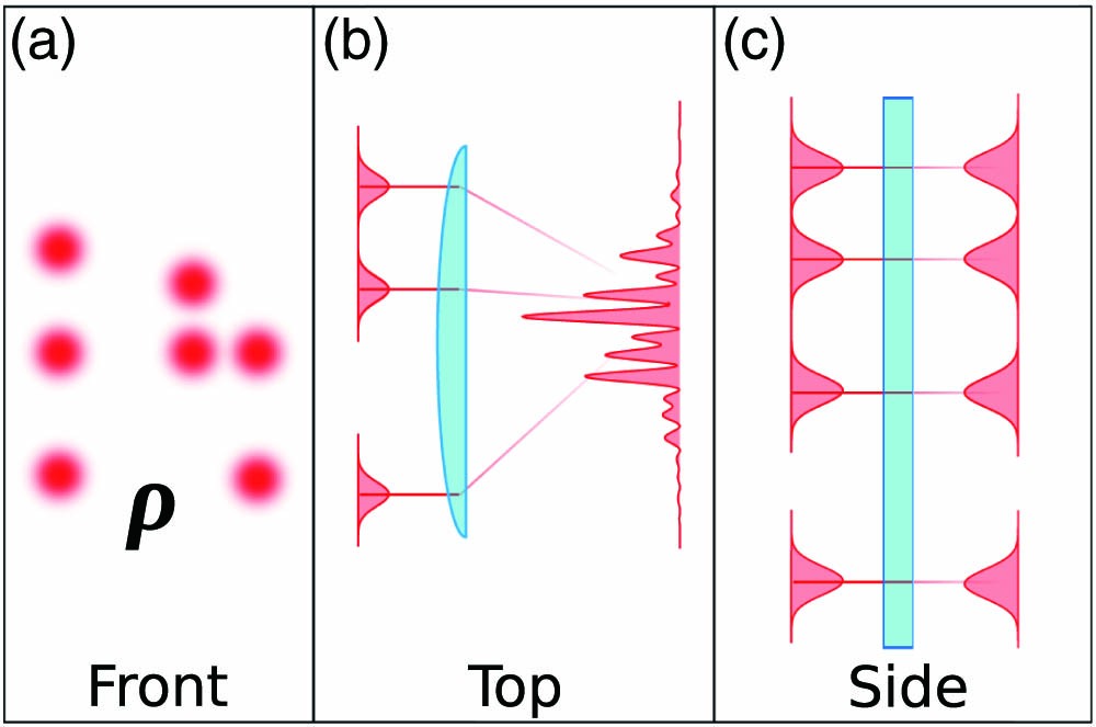
Fig. 1. The working principle of path-encoded quantum state reconstruction. (a) Geometry: the spatial arrangement of paths. (b), (c) Paths passing through a cylindrical lens to an image sensor. Along one direction, the paths are interfered by the lens. Along the other direction, the paths are unaltered. The off-diagonal elements of the density matrix ρ are found by performing a discrete Fourier transform of the recorded interference pattern. The cylindrical lens allows for only chosen sets of paths to be interfered at a time. This allows the method to accommodate duplicate path spacings in the geometry.

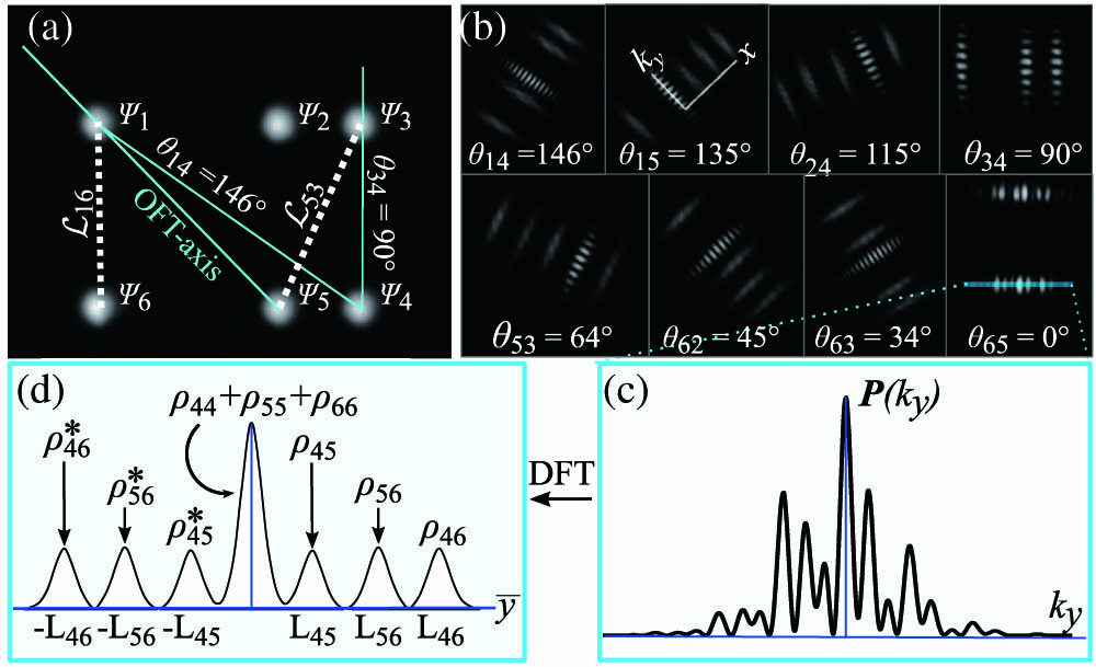
Fig. 2. State reconstruction method. (a) Six paths are shown in the figure and encode the state ρ. The optical Fourier transform (OFT) axis (blue solid line) rotates to particular angles θij, of which a few are shown, to interfere each pair of paths at a time (angles are with respect to a horizontal axis along the bottom-most paths). We assign to each pair of points a line segment Lij. (b) Corresponding OFT for the eight angles required to reconstruct this particular density matrix. As only paths with angle θij between them interfere, the diagonal elements can be recovered from the remaining paths. The ky axis is always in the direction of the interference, and the x axis is perpendicular to it (example shown for θ15). (c) Each pattern is recorded and analyzed one at a time via discrete Fourier transform (DFT) by taking a one pixel wide “slice” through the interference pattern. This process is repeated for every interference pattern present in a given image. (d) Fourier transform of the interference pattern (for illustrative purposes, we plot the magnitude). The magnitude ρij is recovered from the height of the DFT at the position y¯=Lij. The normalization is obtained by summing the zero frequency peaks of each interference pattern present in the θ65 subpanel (in this example) in panel (b). All panels contain real data.

Fig. 3. Experiment demonstrating the state reconstruction method. (a) State preparation in blue box: the Rayleigh length of an 808 nm diode laser is set by a beam expander. A series of displacement crystals (xtal) and half- and quarter-wave plates (labeled by the angles ϕ, ζ, and Ω) generate the state ρ. The resulting eight-path geometry is not compatible with the tomography method, and so two paths are blocked to produce a compatible six-dimensional state. A set of HWP and QWP may be inserted to form a mixed state by rapidly spinning HWPs. The purity is a function of the wave-plate angle τ. We can also produce photon pairs via SPDC at 808 nm using a diode at λ=404  nm to pump a 15 mm ppKTP crystal. The measured g(2)(0) of the source is 0.1979±0.0005. (b) Analysis is presented in the purple box: lenses f1=1000  mm and f2=400  mm image the six paths onto a camera (an electron multiplying CCD in the case of down-converted photons). A rotating cylindrical lens (f=250  mm) performs the optical Fourier transform (OFT) along the OFT axis. A one pixel wide slice of each interference pattern is analyzed with DFT on a computer. Wider slices can be used and averaged over; however, this may reduce the visibility if there are imperfections in the interference pattern. This would include tilting of the dark fringes, or, as can be seen in the figure, if the intensity in each bright fringe is not evenly distributed. The coherences are obtained by the heights of the Fourier transform peaks, normalized by the total intensity. No filters are applied to the raw data.

Fig. 4. Experimental results. (a) Experimental (dots) and theoretical (curves) coherences ρij of the density matrix ρ. These are produced by varying the QWP angle ζ in Fig. 3. As the coherences are constrained by the experimental setup, only a few unique values appear in any given matrix. As such, data points for multiple coherences overlap. Note that error bars, obtained by averaging over multiple pictures, were omitted for clarity but range from 10−3 to 10−2. (b) Experimentally reconstructed six-dimensional state ρ(ζ=30°). Each diagram represents a 6×6 matrix, with theoretical elements to the right of each experimental element. The fidelity with the nominal input state is 0.9911 (fidelity is one if the states are identical).

Fig. 5. Experimental results. (a) Fidelity as a function of the wave-plate angles ϕ, ζ, and Ω, shown in Fig. 3. The fidelity is close to unity, meaning ρ and ρth are nearly equal. Averaged over all points, the fidelity is 0.9852±0.0008 (dashed line). (b) Purity Tr {ρ2} as a function of the HWP angle τ for a classical source and single-photon source. The single-photon source deviates due to the much shorter coherence length. (c) Reconstructed density matrix of single photons in four paths. The experimental values are labeled. The corresponding theoretical values are either 0.25 or 0. The calculated fidelity is 1.00±0.03.