The interaction of relativistically intense laser pulses with solid targets has stimulated considerable interest because of its practical applications in laser-driven particle acceleration^[1–7], high-brightness ultrafast hard X-ray and $\text{K}_{\unicode[STIX]{x1D6FC}}$ source^[8–11], cancer treatment^{[12, 13]}, fast ignition in inertial confinement fusion^[14], etc. A crucial issue, in all these applications, is to produce high-quality forward hot electrons efficiently. Some experimental and simulation results^[15–25] indicate that the interaction of the intense laser pulse with the subwavelength nanowire targets can significantly increase laser energy absorption and enhance the flux and energy of relativistic electrons compared to flat targets. In addition, nanowire arrays can greatly affect the transport of the fast electrons and the generation of mega-ampere relativistic electron beams ^{[17, 26, 27]}. There are also strong magnetic fields (about $100~\text{MG}$) produced within the nanowire arrays^{[20, 27]}. It is worth noting that the self-generated magnetic field plays an important role in both the production and the transport of the fast electrons. However, the mechanism of the generation of the magnetic field in nanostructured arrays has not yet been studied in detail.

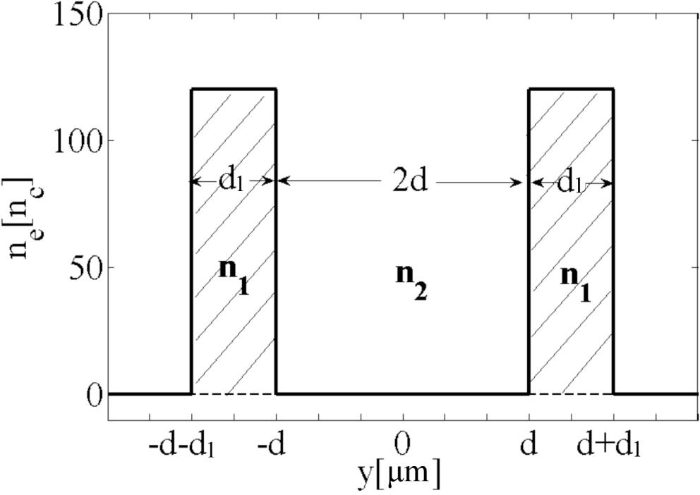
In this paper, we consider an ultra-intense laser pulse normally irradiating on a fully ionized nanolayered target. The schematic diagram of the electron density for the nanolayered target (partial) is shown in Figure 1. Since the averaged electron density of the nanolayered target is much larger than the critical density $n_{c}$, the interaction of the laser pulse with the nanolayered target mainly occurs near the front surface of the target. Here, $n_{c}=m_{e}\unicode[STIX]{x1D700}_{0}\unicode[STIX]{x1D714}_{0}^{2}/e^{2}$ is the critical density; $m_{e}$, $-e$, $\unicode[STIX]{x1D700}_{0}$ and $\unicode[STIX]{x1D714}_{0}$ represent the electron mass, electron charge, dielectric constant in vacuum and laser angular frequency, respectively. During the interaction of the laser pulse with the nanolayered target, a large number of energetic electrons are accelerated by the laser pulse, resulting in the formation of a relativistic electron beam. At relativistic intensities, $10^{18}{-}10^{22}~\text{W}/\text{cm}^{2}$, most of the laser energy is transported by relativistic electrons, which are collisionless. Charge neutrality requires that a flux of relativistic electron beam into the target must be balanced by a return current of thermal electrons. Note that the returned thermal electrons are reflected by the sheath field at the interface of the nanolayered target while the relativistic electrons can spread inside the target with a divergence angle, resulting in a net current along the surface of the nanolayered structure. Thus, quasi-static magnetic fields of the order of $100~\text{MG}$ can be produced inside the gaps between the nanolayers.

If the laser spot size is large enough, we can simply assume that an equally infinite and uniform fast electron beam with electron density $n_{h}$ and averaged velocity $v_{h}$ propagates along the $x$-axis. The neutralizing electron current also flows in the $x$-direction with averaged velocity $v_{e0}$. Since magnetic fields can develop in a very short time, the combined system of the fast electron beam and the response of the background plasma can be suitably treated by a single-fluid electron magneto-hydrodynamic (EMHD) description, which contains electron-fluid equations and Maxwell equations. The electron-fluid equations consist of the continuity equation and the force balance equation. From it, we can obtain the relationship between the self-generated magnetic field and the electron flow velocity as^{[28, 29]}1$$\begin{eqnarray}\displaystyle \mathbf{B}={\displaystyle \frac{c}{e}}\unicode[STIX]{x1D6FB}\times \mathbf{p}_{e}, & & \displaystyle\end{eqnarray}$$ where $\mathbf{p}_{e}=m_{e}\unicode[STIX]{x1D6FE}_{e}\mathbf{v}_{e0}$ is the momentum of the background electrons, $\unicode[STIX]{x1D6FE}_{e}$ is the relativistic factor, $-e$ is the electron charge and $c$ is the speed of light. Besides, the self-generated electromagnetic fields in the nanolayered target satisfy the Maxwell equations 2$$\begin{eqnarray}\displaystyle \unicode[STIX]{x1D6FB}\times \mathbf{B}={\displaystyle \frac{4\unicode[STIX]{x1D70B}}{c}}(-en_{e}\mathbf{p}_{e}/m_{e}\unicode[STIX]{x1D6FE}_{e}+\mathbf{j}_{h})+{\displaystyle \frac{1}{c}}{\displaystyle \frac{\unicode[STIX]{x2202}\mathbf{E}}{\unicode[STIX]{x2202}t}}, & & \displaystyle\end{eqnarray}$$ where $\mathbf{j}_{h}$ is the current density of the fast electron beam and $n_{e}$ is the background electron density. Here, for a long beam with pulse length $l_{b}\gg v_{h}/\unicode[STIX]{x1D714}_{p}$, where $v_{h}$ and $\unicode[STIX]{x1D714}_{p}$ are the fast electron beam velocity and background plasma frequency, the displacement current $(1/c)(\unicode[STIX]{x2202}\mathbf{E}/\unicode[STIX]{x2202}t)$ is of order $(v_{h}/\unicode[STIX]{x1D714}_{p}l_{b})\ll 1$ compared to the electron current. So, the displacement current can be neglected. Equation (2) can be rewritten as 3$$\begin{eqnarray}\displaystyle \mathbf{p}_{e}=-{\displaystyle \frac{m_{e}c\unicode[STIX]{x1D6FE}_{e}}{4\unicode[STIX]{x1D70B}en_{e}}}\unicode[STIX]{x1D6FB}\times \mathbf{B}+{\displaystyle \frac{m_{e}\unicode[STIX]{x1D6FE}_{e}}{e}}{\displaystyle \frac{\mathbf{j}_{h}}{n_{e}}}. & & \displaystyle\end{eqnarray}$$ Substituting Equation (3) into Equation (1), we can obtain 4$$\begin{eqnarray}\mathbf{B}={\displaystyle \frac{m_{e}c}{e^{2}}}\left({\displaystyle \frac{1}{n_{e}}}\unicode[STIX]{x1D6FB}\times \mathbf{j}_{h}-{\displaystyle \frac{1}{n_{e}^{2}}}\unicode[STIX]{x1D6FB}n_{e}\times \mathbf{j}_{h}\right)-\unicode[STIX]{x1D6FB}\times (\unicode[STIX]{x1D6FF}_{pe}^{2}\unicode[STIX]{x1D6FB}\times \mathbf{B}),\end{eqnarray}$$ where $\unicode[STIX]{x1D6FF}_{pe}=c/\unicode[STIX]{x1D714}_{pe}$ is the electron skin depth and $\unicode[STIX]{x1D714}_{pe}=(4\unicode[STIX]{x1D70B}n_{e}e^{2}/m_{e})^{1/2}$ is the electron plasma frequency. The three terms of the right-hand side of Equation (4) are the source of the self-generated magnetic field. The first term generates a magnetic field that pushes the fast electrons toward regions of higher fast electron current density, and the second term pushes the fast electrons toward regions of lower density. The third term represents the interaction of the self-generated magnetic field with the plasmas of the nanolayered target. From Equation (4), it is obvious that a sharp electron density gradient and a strong fast electron current are necessary to generate a strong magnetic field. For the nanolayered target, in order to keep the charge neutrality, the return electrons must exist inside the nanolayers. Due to the strong self-generated magnetic field, most of the fast electrons and return electrons are bounded near the edges of the nanolayers.

To further understand the characteristics of the self-generated magnetic fields, we take a part of the nanolayered target as an example to analyze the generation of the magnetic field when the laser pulse interacts with the nanolayered target. As shown in Figure 1, three regions are divided as follows: region 1 with $-d_{1}-d and the region 3 with $d are the high-density plasma for the nanolayers and region 2 with $-d is the gap between the nanolayers. In order to solve Equation (4), a one-dimensional model is adopted to quantitatively estimate the self-generated magnetic field. In other words, only the spatial variations in the $y$-direction are considered. Then, Equation (4) can be rewritten as 5$$\begin{eqnarray}\left\{\begin{array}{@{}l@{}}-\unicode[STIX]{x1D6FF}_{pe1}^{2}{\displaystyle \frac{\unicode[STIX]{x2202}^{2}}{\unicode[STIX]{x2202}y^{2}}}\mathbf{B}+\mathbf{B}=0,\quad -d-d_{1} where $d_{1}$ is the width of the nanolayer, $\unicode[STIX]{x1D6FF}_{pei}=c/\unicode[STIX]{x1D714}_{pei}$ is the electron skin depth and $\unicode[STIX]{x1D714}_{pei}=(4\unicode[STIX]{x1D70B}n_{i}e^{2}/m_{e})^{1/2}$ is the electron plasma frequency for the $i$th region $(i=1,2)$. Here, the electron density $n_{2}$ and the fast electron current density $j_{h}$ are assumed as constants. From Equation (5), the self-generated magnetic field can be solved analytically as follows: 6$$\begin{eqnarray}\mathbf{B}=\left\{\begin{array}{@{}l@{}}c_{1}\mathbf{exp}\left({\displaystyle \frac{y}{\unicode[STIX]{x1D6FF}_{pe1}}}\right)+c_{2}\mathbf{exp}\left({\displaystyle \frac{-y}{\unicode[STIX]{x1D6FF}_{pe1}}}\right),\quad -d-d_{1} The constants $c_{1},c_{2},c_{3},c_{4},c_{5}$ and $c_{6}$ can be solved by the boundary conditions 7$$\begin{eqnarray}\left\{\begin{array}{@{}l@{}}c_{1}={\displaystyle \frac{\mathbf{B}_{0}\mathbf{exp}\left({\displaystyle \frac{d_{1}}{\unicode[STIX]{x1D6FF}_{pe1}}}\right)-\mathbf{B}_{1}}{\mathbf{exp}\left({\displaystyle \frac{-d+d_{1}}{\unicode[STIX]{x1D6FF}_{pe1}}}\right)-\mathbf{exp}\left({\displaystyle \frac{-d-d_{1}}{\unicode[STIX]{x1D6FF}_{pe1}}}\right)}},\\[25.0pt] c_{2}={\displaystyle \frac{\mathbf{B}_{1}-\mathbf{B}_{0}\mathbf{exp}\left({\displaystyle \frac{-d_{1}}{\unicode[STIX]{x1D6FF}_{pe1}}}\right)}{\mathbf{exp}\left({\displaystyle \frac{d+d_{1}}{\unicode[STIX]{x1D6FF}_{pe1}}}\right)-\mathbf{exp}\left({\displaystyle \frac{d-d_{1}}{\unicode[STIX]{x1D6FF}_{pe1}}}\right)}},\\[25.0pt] c_{3}={\displaystyle \frac{-\mathbf{B}_{0}\mathbf{exp}\left(-{\displaystyle \frac{d}{\unicode[STIX]{x1D6FF}_{pe2}}}\right)+\mathbf{B}_{1}\mathbf{exp}\left({\displaystyle \frac{d}{\unicode[STIX]{x1D6FF}_{pe2}}}\right)}{\mathbf{exp}\left({\displaystyle \frac{2d}{\unicode[STIX]{x1D6FF}_{pe2}}}\right)-\mathbf{exp}\left(-{\displaystyle \frac{2d}{\unicode[STIX]{x1D6FF}_{pe2}}}\right)}},\\[25.0pt] c_{4}={\displaystyle \frac{\mathbf{B}_{0}\mathbf{exp}\left({\displaystyle \frac{d}{\unicode[STIX]{x1D6FF}_{pe2}}}\right)-\mathbf{B}_{1}\mathbf{exp}\left(-{\displaystyle \frac{d}{\unicode[STIX]{x1D6FF}_{pe2}}}\right)}{\mathbf{exp}\left({\displaystyle \frac{2d}{\unicode[STIX]{x1D6FF}_{pe2}}}\right)-\mathbf{exp}\left(-{\displaystyle \frac{2d}{\unicode[STIX]{x1D6FF}_{pe2}}}\right)}},\\[25.0pt] c_{5}={\displaystyle \frac{\mathbf{B}_{0}-\mathbf{B}_{1}\mathbf{exp}\left({\displaystyle \frac{-d_{1}}{\unicode[STIX]{x1D6FF}_{pe1}}}\right)}{\mathbf{exp}\left({\displaystyle \frac{d+d_{1}}{\unicode[STIX]{x1D6FF}_{pe1}}}\right)-\mathbf{exp}\left({\displaystyle \frac{d-d_{1}}{\unicode[STIX]{x1D6FF}_{pe1}}}\right)}},\\[25.0pt] c_{6}={\displaystyle \frac{\mathbf{B}_{1}\mathbf{exp}\left({\displaystyle \frac{d_{1}}{\unicode[STIX]{x1D6FF}_{pe1}}}\right)-\mathbf{B}_{0}}{\mathbf{exp}\left({\displaystyle \frac{-d+d_{1}}{\unicode[STIX]{x1D6FF}_{pe1}}}\right)-\mathbf{exp}\left({\displaystyle \frac{-d-d_{1}}{\unicode[STIX]{x1D6FF}_{pe1}}}\right)}},\end{array}\right.\end{eqnarray}$$ where $\mathbf{B}_{0}$ and $\mathbf{B}_{1}$ are the maximum magnetic fields at the nanolayer interfaces ($y=-d$ and $y=d$). Note that $n_{1}\gg n_{2}$, $d_{1}\gg \unicode[STIX]{x1D6FF}_{pe1}$ and $d\gg \unicode[STIX]{x1D6FF}_{pe2}$ in the nanolayered target. In order to get the values of $\mathbf{B}_{0}$ and $\mathbf{B}_{1}$, we integrate Equation (4) across the interfaces of $y=-d$ and $y=d$. Then, we can obtain the integrated magnetic flux^{[30, 31]}8$$\begin{eqnarray}\left\{\begin{array}{@{}l@{}}\unicode[STIX]{x1D6F7}_{0}=(\unicode[STIX]{x1D6FF}_{pe1}+\unicode[STIX]{x1D6FF}_{pe2})\mathbf{B}_{0}={\displaystyle \frac{m_{e}c}{e^{2}}}\left({\displaystyle \frac{\mathbf{j}_{h2}}{n_{2}}}-{\displaystyle \frac{\mathbf{j}_{h1}}{n_{1}}}\right),\\[15.0pt] \unicode[STIX]{x1D6F7}_{1}=(\unicode[STIX]{x1D6FF}_{pe1}+\unicode[STIX]{x1D6FF}_{pe2})\mathbf{B}_{1}={\displaystyle \frac{m_{e}c}{e^{2}}}\left({\displaystyle \frac{\mathbf{j}_{h3}}{n_{1}}}-{\displaystyle \frac{\mathbf{j}_{h2}}{n_{2}}}\right),\end{array}\right.\end{eqnarray}$$ where $\unicode[STIX]{x1D6F7}_{0}=\int _{-d-d_{1/2}}^{0}\mathbf{B}\,\text{d}y$, $\unicode[STIX]{x1D6F7}_{1}=\int _{0}^{d+d_{1/2}}\mathbf{B}\,\text{d}y$ are the integrated magnetic fluxes and $\mathbf{j}_{hi}=en_{hi}v_{hi}$$(i=1,2,3)$ are the electron current densities within different regions. Since the background electron density satisfies $n_{1}\gg n_{2}$ and the fast electron current densities are assumed as $\mathbf{j}_{h}\simeq \mathbf{j}_{h1}\simeq \mathbf{j}_{h2}\simeq \mathbf{j}_{h3}$, the terms $\mathbf{j}_{h1}/n_{1}$ and $\mathbf{j}_{h3}/n_{3}$ can be neglected in Equation (8). Then, we can obtain 9$$\begin{eqnarray}\left\{\begin{array}{@{}l@{}}\mathbf{B}_{0}={\displaystyle \frac{m_{e}c}{e^{2}(\unicode[STIX]{x1D6FF}_{pe1}+\unicode[STIX]{x1D6FF}_{pe2})}}{\displaystyle \frac{\mathbf{j}_{h}}{n_{2}}},\\[15.0pt] \mathbf{B}_{1}=-{\displaystyle \frac{m_{e}c}{e^{2}(\unicode[STIX]{x1D6FF}_{pe1}+\unicode[STIX]{x1D6FF}_{pe2})}}{\displaystyle \frac{\mathbf{j}_{h}}{n_{2}}}.\end{array}\right.\end{eqnarray}$$

If we simply assume that the absorbed laser energy flux is approximately equal to the electron energy flux $\unicode[STIX]{x1D701}I_{18}=0.02fn_{h}T_{\text{keV}}^{3/2}$ [32], where the electron temperature is expressed by the ‘Beg law’^[33] with $T_{\text{keV}}=200I_{18}^{1/3}$, $n_{h}=\unicode[STIX]{x1D701}I_{18}/(0.02fT_{\text{keV}}^{3/2})$ is the density of energy carrying electrons in units of $10^{23}~\text{cm}^{-3}$, $\unicode[STIX]{x1D701}$ is the fraction of laser energy absorbed by the fast electrons and $f$ is the flux limiting factor. Here, the ratio of $\unicode[STIX]{x1D701}$ to $f$ is approximated as $\unicode[STIX]{x1D701}/f=0.39$. Thus, the maximum value for the magnetic field can be written as 10$$\begin{eqnarray}\text{B}_{max}=188{\displaystyle \frac{\unicode[STIX]{x1D701}}{f}}{\displaystyle \frac{I_{18}^{1/2}}{\left(1\bigg/\sqrt{{\displaystyle \frac{n_{1}}{n_{c}}}}+1\bigg/\sqrt{{\displaystyle \frac{n_{2}}{n_{c}}}}\right){\displaystyle \frac{n_{2}}{n_{c}}}}}{\displaystyle \frac{v_{h}}{c}}\,\text{MG},\end{eqnarray}$$ where $v_{h}\simeq c$ is the fast electron velocity, $n_{1}$ is the electron density of the nanolayers, $n_{2}$ is the electron density in the gaps between the nanolayers, $n_{c}=m_{e}\unicode[STIX]{x1D700}_{0}\unicode[STIX]{x1D714}_{0}^{2}/e^{2}$ is the critical density and $I_{18}^{1/2}$ is the normalized laser intensity.

Substituting Equation (7) into Equation (6) and combining Equation (9), we can obtain the complete expression of the self-generated magnetic field in the transverse direction. It can be found that the self-generated magnetic field is strongly dependent on the sharp gradient of the plasma density near the nanolayer interfaces ($y=\pm 0.3~\unicode[STIX]{x03BC}\text{m}$) and the current density of the fast electrons. Figure 2(a) shows the magnetic field generated in the nanolayered target with different electron densities $n_{2}=2n_{c},4n_{c},10n_{c}$ (in the nanolayered gap). The initial plasma density of the nanolayers is $n_{1}=120n_{c}$ and the current density of the fast electron is assumed as $j_{h}=3n_{c}ec$. The width of the nanolayers is $d_{1}=0.2~\unicode[STIX]{x03BC}\text{m}$ and the width of the gap between the nanolayers is $2d=0.6~~\unicode[STIX]{x03BC}\text{m}$. It can be clearly seen that the maximum value of the self-generated magnetic field is present near the nanolayer interfaces $y=\pm 0.3~\unicode[STIX]{x03BC}\text{m}$ with the values of $B_{0}$ and $B_{1}$. The intensity of the self-generated magnetic field decreases as the nanolayered gap plasma density ($n_{2}$) increases due to the decrease of the plasma density gradient near the nanolayer interface. It is clear that the magnetic field exists within the skin depth $\unicode[STIX]{x1D6FF}_{pe}$, so the magnetic field decays rapidly to zero in the nanolayer region. And due to the lower electron density in the nanolayered gap, the magnetic field decays much slower than that in the nanolayer region. Figure 2(b) shows the magnetic fields generated in the nanolayered target with different fast electron current densities of $j_{h}=1n_{c}ec,3n_{c}ec,5n_{c}ec$. The electron density in the nanolayered gap is $1n_{c}$. The other parameters are similar to those in Figure 2(a). We found that with the same plasma density gradient near the nanolayer interfaces ($y=\pm 0.3~\unicode[STIX]{x03BC}\text{m}$), the maximum intensity of the self-generated magnetic field increases as the fast electron current density ($j_{h}$) increases. The physical reason is clear that the higher fast electron current density could induce higher return current density, which in turn makes the self-generated magnetic field much stronger. In addition, the theoretical analysis does not consider the detailed interaction process between the laser pulse with the nanolayered target. So, in the theoretical analysis, the width of the nanolayered gap does not affect the maximum intensity of the self-generated magnetic field but only affects the distribution of the self-generated magnetic field.

In the following, the generation of magnetic fields is studied in further detail by the two-dimensional (2D) particle-in-cell (PIC) simulations, which are performed using the simulation code EPOCH^[34]. In simulations, we take p-polarized laser pulses with normalized intensity of $a_{0}=6.0$, which are incident along the $x$-direction. The wavelength and duration of the laser pulse are $\unicode[STIX]{x1D706}_{0}=1~\unicode[STIX]{x03BC}\text{m}$ and $\unicode[STIX]{x1D70F}=330\text{ fs}$, respectively. The laser spot is large enough so that the transverse intensity of the laser pulse is uniform. The simulation box is $15~\unicode[STIX]{x03BC}\text{m}\times 10~\unicode[STIX]{x03BC}\text{m}$ with a resolution of 170 cells per $\unicode[STIX]{x1D706}$ in the longitudinal and transverse directions. The nanolayered target is located from $5~\unicode[STIX]{x03BC}\text{m}$ to $15~\unicode[STIX]{x03BC}\text{m}$, and the electron density of the nanowires is $120n_{c}$. The gaps between the nanolayers are empty at the initial time. Similar to the structure in Figure 1, the width of the nanolayers is $d_{1}=0.2~\unicode[STIX]{x03BC}\text{m}$ and the width of the nanolayered gap is $2d=0.6~\unicode[STIX]{x03BC}\text{m}$.

During the interaction of the laser pulse with the nanolayered target, most of the laser energy is absorbed by the nanolayered target. And a large number of energetic electrons can be accelerated by the laser pulse. The simulation results indicate that the peak of the laser energy absorption can reach as high as $80\%$. The temperature of the fast electrons calculated from the electron spectrum is about $0.81\text{ MeV}$, which is well consistent with the calculated value $T_{e}=0.79\text{ MeV}$ by the Beg law.

Figure 3(a) shows the magnetic fields produced by the interaction of a laser pulse with the nanolayered target at time $46.7\text{ fs}$. In Fig, 3(a), it can be clearly seen that the strong periodic positive and negative quasi-static magnetic fields are generated near the nanolayer interfaces. In this case, the maximum value of the magnetic field can reach $300~\text{MG}$. Figure 3(b) shows the transverse distribution of self-generated magnetic fields at $x=8~\unicode[STIX]{x03BC}\text{m}$. The blue solid curve is for the simulation result and the black dot curve is for the analytical result. To obtain the analytical result, we have to count the current density $j_{h}$ and electron density $n_{2}$ from the PIC simulation results. The current density $j_{h}=-3.3n_{c}ec$ is counted as the averaged current density of the forward fast electrons at the position $x=8~\unicode[STIX]{x03BC}\text{m}$ and the transverse range of $y=(0,1)~\unicode[STIX]{x03BC}\text{m}$. The electron density of the nanolayered gap $n_{2}=0.7n_{c}$ is counted as the averaged background electron density at the position $x=8~\unicode[STIX]{x03BC}\text{m}$ and the transverse range of $y=(0.2,0.8)~\unicode[STIX]{x03BC}\text{m}$. The velocity of the fast electrons is approximately assumed as $v_{h}\simeq c$. Then the transverse distribution of self-generated magnetic fields can be obtained by using Equation (6). We can see that the simulation result is well consistent with the analysis result. The slight difference of the self-generated magnetic field between the analytical result and the PIC simulation is only at the position of the nanolayered gap. Here, the distribution of the self-generated magnetic field is affected by the distribution of electron density in the nanolayered gap. In the analytical model, the distribution of electron density of the nanolayered gap is counted as a uniform value. But, in PIC simulation results, the distribution of the electron density near the nanolayers could be higher than that away from the nanolayers. So the slight difference of the self-generated magnetic field in the nanolayered gap is mainly caused by the nonuniform electron density.

In the theoretical analysis, the current density of the fast electron beam could affect the intensity of the self-generated magnetic field. So, we can change the intensity of the laser pulse to affect the current density of the fast electron beam and thus the intensity of the self-generated magnetic field. In Figure 4, we plot the maximum intensity of the self-generated magnetic field versus the normalized intensity of the laser pulse. The blue dashed line stands for the simulation results and the black solid line stands for the theoretical analysis results by using Equation (10). In the analytical model, the velocity of the fast electrons is approximately assumed as $v_{h}\simeq c$, and the electron density of the nanolayers is $n_{1}=120n_{c}$; the electron density of the nanolayered gap is approximately $n_{2}=1n_{c}$, and the ratio of $\unicode[STIX]{x1D701}$ to $f$ is approximated as $\unicode[STIX]{x1D701}/f=0.39$. In simulations, except for the laser intensity, the other laser and plasma parameters are the same as in Figure 3(a). In Figure 4, it can be seen that the simulation results and the analytical results are basically consistent.

In summary, we have established accurate results for the generation of magnetic fields in a laser irradiated nanolayered target based on the EMHD approximation. The resultant structure and amplitude of the magnetic field inside the nanolayered target are determined for a given laser intensity and plasma density. It reveals that the characteristics of the self-generated magnetic field are strongly dependent on the density gradient of the nanostructured arrays and the fast electron current. The 2D-PIC simulation results are in good agreement with the theoretical analysis. When designing the relevant experiments of the interaction of ultra-intense laser pulse with a nanowire target, our work can better predict the structure and the intensity of the self-generated magnetic field inside the nanowire target, which is beneficial to improving the quality of the energetic electrons and ions accelerated by the laser pulse in the nanowire target.

References

[1] J. Faure, C. Rechatin, A. Norlin, A. Lifschitz, Y. Glinec, V. Malka. Nature, 444, 737(2006).
[2] A. Macchi, M. Borghesi, M. Passoni. Rev. Mod. Phys., 85, 751(2013).
[3] F. Wagner, C. Brabetz, O. Deppert, M. Roth, T. Stohlker, An. Tauschwitz, A. Tebartz, B. Zielbauer, V. Bagnoud. High Power Laser Sci. Eng., 4, e45(2016).
[4] S. Kawata, T. Nagashima, M. Takano, T. Izumiyama, D. Kamiyama, D. Barada, Q. Kong, Y. J. Gu, P. X. Wang, Y. Y. Ma, W. M. Wang, W. Zhang, J. Xie, H. R. Zhang, D. B. Dai. High Power Laser Sci. Eng., 2, e4(2014).
[5] J. Schreiber, F. Bell, Z. Najmudin. High Power Laser Sci. Eng., 2, e41(2014).
[6] D. Khaghani, M. Lobet, B. Borm, L. Burr, F. Gartner, L. Gremillet, L. Movsesyan, O. Rosmej, M. E. Toimil-Molares, F. Wagner, P. Neumayer. Sci. Rep., 7, 11366(2017).
[7] M. Dozires, G. M. Petrov, P. Forestier-Colleoni, P. Campbell, K. Krushelnick, A. Maksimchuk, C. McGuffey, V. Kaymak, A. Pukhov, M. G. Capeluto, R. Hollinger, V. N. Shlyaptsev, J. J. Rocca, F. N. Beg. Plasma Phys. Control. Fusion, 61(2019).
[8] A. Rousse, C. Rischel, J.-C. Gauthier. Rev. Mod. Phys., 73, 17(2001).
[9] A. Pukhov. Nat. Phys., 2, 439(2006).
[10] L. M. Chen, F. Liu, W. M. Wang, M. Kando, J. Y. Mao, L. Zhang, J. L. Ma, Y. T. Li, S. V. Bulanov, T. Tajima, Y. Kato, Z. M. Sheng, Z. Y. Wei, J. Zhang. Phys. Rev. Lett., 104(2010).
[11] E. Brambrink, S. Baton, M. Koenig, R. Yurchak, N. Bidaut, B. Albertazzi, J. E. Cross, G. Gregori, A. Rigby, E. Falize, A. Pelka, F. Kroll, S. Pikuz, Y. Sakawa, N. Ozaki, C. Kuranz, M. Manuel, C. Li, P. Tzeferacos, D. Lamb. High Power Laser Sci. Eng., 4, e30(2016).
[12] V. Malka, S. Fritzler, E. Lefebvre, E. dHumieres, R. Ferrand, G. Grillon, C. Albaret, S. Meyroneinc, J.-P. Chambaret, A. Antonetti, D. Hulin. Med. Phys., 31, 1587(2004).
[13] D. Schardt. Nucl. Phys. A, 787, 633(2007).
[14] M. Tabak, J. Hammer, M. E. Glinsky, W. L. Kruer, S. C. Wilks, J. Woodworth, E. M. Campbell, M. D. Perry, R. J. Mason. Phys. Plasmas, 1, 1626(1994).
[15] A. Moreau, R. Hollinger, C. Calvi, S. Wang, Y. Wang, M. G. Capeluto, A. Rockwood, A. Curtis, S. Kasdorf, V. N. Shlyaptsev, V. Kaymak, A. Pukhov, J. J. Rocca. Plasma Phys. Control. Fusion, 62(2020).
[16] D. Sarkar, P. K. Singh, G. Cristoforetti, A. Adak, G. Chatterjee, M. Shaikh, A. D. Lad, P. Londrillo. Appl. Phys. Lett. Photonics, 2(2017).
[17] A. Curtis, C. Calvi, J. Tinsley, R. Hollinger, V. Kaymak, A. Pukhov, S. J. Wang, A. Rockwood, Y. Wang, V. N. Shlyaptsev, J. J. Rocca. Nat. Commun., 9, 1077(2018).
[18] M. A. Purvis, V. N. Shlyaptsev, R. Hollinger, C. Bargsten, A. Pukhov, A. Prieto, Y. Wang, B. M. Luther, L. Yin, S. Wang, J. J. Rocca. Nat. Photonics, 7, 796(2013).
[19] Z. Q. Zhao, L. H. Cao, L. F. Cao, J. Wang, W. Z. Huang, W. Jiang, Y. L. He, Y. C. Wu, B. Zhu, K. G. Dong, Y. K. Ding, B. H. Zhang, Y. Q. Gu, M. Y. Yu, X. T. He. Phys. Plasmas, 17(2010).
[20] V. Kaymak, A. Pukhov, V. N. Shlyaptsev, J. J. Rocca. Phys. Rev. Lett., 117(2016).
[21] L. H. Cao, Y. Q. Gu, Z. Q. Zhao, L. F. Cao, W. Z. Huang, W. M. Zhou, H. B. Cai, X. T. He, W. Yu, M. Y. Yu. Phys. Plasmas, 17(2010).
[22] L. H. Cao, Y. Q. Gu, Z. Q. Zhao, L. F. Cao, W. Z. Huang, W. M. Zhou, X. T. He, W. Yu, M. Y. Yu. Phys. Plasmas, 17(2010).
[23] J. Q. Yu, W. M. Zhou, L. H. Cao, Z. Q. Zhao, L. F. Cao, L. Q. Shan, D. X. Liu, X. L. J, B. Li, Y. Q. Gu. Appl. Phys. Lett., 100(2012).
[24] L. L. Ji, S. Jiang, A. Pukhov, R. Freeman, K. Akli. High Power Laser Sci. Eng., 5(2017).
[25] S. Jiang, L. L. Ji, H. Audesirk, K. M. George, J. Snyder, A. Krygier, P. Poole, C. Willis, R. Daskalova, E. Chowdhury, N. S. Lewis, D.W. Schumacher, A. Pukhov, R. R. Freeman, K. U. Akli. Phys. Rev. Lett., 116(2016).
[26] P. K. Singh, G. Chatterjee, A. D. Lad, A. Adak, S. Ahmed, M. Khorasaninejad, M. M. Adachi, K. S. Karim, S. S. Saini, A. K. Sood, G. Ravindra Kumar. Appl. Phys. Lett., 100(2012).
[27] G. Chatterjee, P. K. Singh, S. Ahmed, A. P. L. Robinson, A. D. Lad, S. Mondal, V. Narayanan, I. Srivastava, N. Koratkar, J. Pasley, A. K. Sood, G. R. Kumar. Phys. Rev. Lett., 108(2012).
[28] E. A. Startsev, R. C. Davidson, M. Dorf. Phys. Plasmas, 16(2009).
[29] H. B. Cai, S. P. Zhu, M. Chen, S. Z. Wu, X. T. He, K. Mima. Phys. Rev. E, 83(2011).
[30] A. R. Bell, J. R. Davies, S. M. Guerin. Phys. Rev. E, 58, 2471(1998).
[31] W. S. Zhang, H. B. Cai, S. P. Zhu. Phys. Plasmas, 22(2015).
[32] A. B. Bell, A. P. L. Robinson, M. Sherlock, R. J. Kingham, W. Rozmus. Plasma Phys. Control. Fusion, 48(2006).
[33] F. N. Beg, A. R. Bell, A. E. Dangor, C. N. Danson, A. P. Fews, M. E. Glinsky, B. A. Hamme, P. Lee, P. A. Norreys, M. Tatarakis. Phys. Plasmas, 4, 447(1997).
[34] T. D. Arber, K. Bennett, C. S. Brady, A. Lawrence-Douglas, M. G. Ramsay, N. J. Sircombe, P. Gillies, R. G. Evans, H. Schmitz, A. R. Bell, C. P. Ridgers. Plasma Phys. Control. Fusion, 57(2015).
J. M. Tian, H. B. Cai, W. S. Zhang, E. H. Zhang, B. Du, S. P. Zhu. Generation mechanism of 100 MG magnetic fields in the interaction of ultra-intense laser pulse with nanostructured target[J]. High Power Laser Science and Engineering, 2020, 8(2): 02000e16
Download Citation