Noniterative spatially partially coherent diffractive imaging using pinhole array mask

Xingyuan Lu; Yifeng Shao; Chengliang Zhao; Sander Konijnenberg; Xinlei Zhu; Ying Tang; Yangjian Cai; H. Paul Urbach

doi:10.1117/1.AP.1.1.016005

Abstract

We propose and experimentally demonstrate a noniterative diffractive imaging method for reconstructing the complex-valued transmission function of an object illuminated by spatially partially coherent light from the far-field diffraction pattern. Our method is based on a pinhole array mask, which is specially designed such that the correlation function in the mask plane can be obtained directly by inverse Fourier transforming the diffraction pattern. Compared to the traditional iterative diffractive imaging methods using spatially partially coherent illumination, our method is noniterative and robust to the degradation of the spatial coherence of the illumination. In addition to diffractive imaging, the proposed method can also be applied to spatial coherence property characterization, e.g., free-space optical communication and optical coherence singularity measurement.

Keywords

coherent diffractive imaging noniterative method partial coherence pinhole array mask

1 Introduction

Coherent diffractive imaging (CDI) is an important tool for reconstructing the complex-valued transmission function of an object from the far-field diffraction pattern and has been widely applied in material and biological sciences.¹^,² Miao et al.³ first experimentally realized imaging of submicrometer sized noncrystalline specimen using CDI. Many CDI approaches have been developed in the past decades; they can be divided into two types: the iterative methods⁴^–⁹ and the noniterative methods.¹⁰^–¹⁴ However, most of the traditional CDI methods cannot be directly applied to using spatially partially coherent illumination without a proper modification, which hence have limited applications at short wavelengths, e.g., in the x-ray and electron regime, or in the unstable experimental environment. For example, the degradation of the spatial coherence may also be caused by the mechanical movement of the sample and the experimental setup, or by the fluctuation of the ambient medium, e.g., atmospheric turbulence.¹⁵^–¹⁷

Iterative algorithms retrieve the complex-valued transmission function of an object by propagating the field back-and-forth between the object plane and the far-field diffraction plane, and imposing constraints on the field in both planes. Gerchberg and Saxton pioneered the iterative algorithms in 1972 by proposing a straightforward method using two intensities measured in the object plane and in the far-field, respectively.⁴ Iterative algorithms using only one intensity measurement of the far-field diffraction pattern, as proposed by Fienup,⁵^,⁶ require prior knowledge of the support of the object for imposing the support constraint in the object plane. Recently, ptychographic algorithms have become an essential technique for imaging nanoscale objects using short-wavelength sources.⁸ The key feature is that illumination areas at the neighboring shift positions must overlap, and this overlap improves the convergence of the ptychographic algorithms.⁷^,⁸ Recent developments in ptychography allow for simultaneous reconstruction of the probe. This significantly reduces the complexity of experimental setup compared to other CDI methods.⁹

For spatially partially coherent illumination, the propagation of light is described using the mutual coherence function (MCF) instead of the field. Many efforts have been spent to adapt CDI methods to spatially partially coherent illumination.¹⁵^–²⁴ The modification of the iterative algorithms was first reported by Whitehead et al.¹⁵ using mode decomposition of the MCF.¹⁶ Later, ptychographic algorithms have also been modified to work for spatially partially coherent illumination by decomposing the MCF into orthogonal modes.¹⁷^–²¹ Thibault and Menzel¹⁷ proposed a mixed state model from the quantum perspective, which effectively deals with a series of multistate mixing problems including partially coherent illumination and enables more applications of ptychography, such as continuous-scan ptychography¹⁸ and dynamic imaging of a vibrating sample.¹⁹ Furthermore, ptychographic imaging with the simultaneous presence of both multiple probe and multiple object states was also demonstrated.²¹ However, the accuracy of mode decomposition relies on the number of modes for accurately representing the MCF, and it increases as the spatial coherence of the illumination decreases.

Sign up for Advanced Photonics TOC. Get the latest issue of Advanced Photonics delivered right to you！Sign up now

Compared to iterative methods, noniterative methods¹⁰^,¹¹^,¹⁴ do not suffer from issues such as stagnation or nonuniqueness of the solution to the diffractive imaging problem, especially when the illumination becomes spatially partially coherent.²¹^,²⁴ In holographic methods, the field transmitted by the object is perturbed such that the object’s transmission function can be directly extracted from the inverse Fourier transform of the diffraction pattern.¹⁴ This perturbation can be achieved by introducing a pinhole, e.g., Fourier transform holography (FTH),²⁵^–²⁷ or by changing the transmission function at a point of the object, e.g., Zernike quantitative phase imaging.²⁸ The performance of applying holographic methods to spatially partially coherent illumination has been discussed in Ref. 14. Alternative methods extract the object information from the three-dimensional autocorrelation functions obtained by inverse Fourier transforming the three-dimensional data set (e.g., the data set measured by varying focus¹² or another optical parameter¹³).

It has been demonstrated that using noniterative methods can avoid errors due to truncating the number of the modes for representing the MCF.¹²^–¹⁴ However, the degree of the spatial coherence of the illumination limits the field of view (FOV) of the reconstructed object. To be precise, what is reconstructed is a product of the object’s transmission function and a correlation function of the illumination. This correlation function has a maximum at the perturbation point, and its value decreases at a rate that depends on the degree of spatial coherence, as the distance between the perturbation point and the observation point increases. Therefore, the lower the illumination’s degree of spatial coherence is, the smaller the region of the object that can be reconstructed reliably.

In this paper, we propose a noniterative method based on a pinhole array mask (PAM). We place the PAM between the object and the detector, and we measure the far-field diffraction pattern of the spatially partially coherent field transmitted by the PAM. The PAM consists of a periodic array of measurement pinholes and an extra reference pinhole, which is analogous to the perturbation point in FTH.¹⁴ It forms an interference between fields transmitted by the reference pinhole and by the measurement pinholes, and we can directly retrieve the correlation function of the incident light with respect to the reference pinhole at the locations of the measurement pinholes from the interference pattern.

In FTH, since the reference pinhole is placed far from the measurement window, the FOV is rather small due to the low correlation. Our method is advantageous compared to FTH, because splitting the measurement window into a periodic array of measurement pinholes keeps the reference pinhole close to all measurement pinholes and thus maintains a high correlation that results in a large FOV.

Our method places the object at a certain distance before the PAM, instead of superposing the object with the PAM. In practice, this not only offers flexibility for arranging the experimental setup but also allows us to adjust the sampling of the reconstructed object. When the propagation distance satisfies the condition for Fresnel or Fraunhofer diffraction, an object with finite support can be reconstructed from the retrieved correlation function, and its sampling is related to the sampling of the PAM by the Shannon–Nyquist sampling theorem.

Because our method reconstructs the product of the object’s transmission function and the illumination’s correlation function and hence can be used not only for object reconstruction but also for characterization of the spatial coherence structure, it is useful for a broad range of applications in coherent optics, such as the measurement of optical coherence singularity²⁹^,³⁰ and free-space optical communication through turbulent media.³¹^,³²

2 Methods

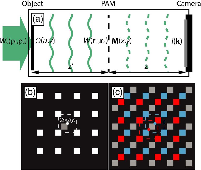
The schematic plot of the experimental setup of our method is shown in Fig. 1, which shows that a transmissive object is illuminated by spatially partially coherent light. In our method, unlike traditional CDI algorithms, we place a PAM between the object and the detector. The location of the PAM is chosen such that light propagation from the object to the PAM and from the PAM to detector obeys either Fresnel or Fraunhofer propagation and hence can be described using Fourier transforms. By doing so, we can divide our method into two steps: (1) retrieving the correlation function of incident light in the PAM plane using a noniterative approach and (2) reconstructing the product of the object’s transmission function and the illumination’s correlation function using a differential method, which requires two diffraction patterns corresponding to the object with and without transmission perturbation, respectively. It is worth noting that the use of this differential method is not necessary for completely spatially coherent illumination.

$Schematic plot of the experimental setup and the concept of the noniterative diffractive imaging method. (a) A PAM is placed between the object and the camera. The PAM is specially designed such that we can retrieve the correlation function of the incident light by inverse Fourier transform of the measured diffraction pattern. (b) The PAM consists of a reference pinhole at the origin (gray square) and a periodic array of the measurement pinholes with certain offset (white squares). (c) In the inverse Fourier transform of the diffraction pattern, the autocorrelation terms (gray squares) and the two interference terms (red and blue squares) are separated by the offset. Each interference term directly contains the correlation between the fields at the reference pinhole and at the measurement pinholes.$

Figure 1.Schematic plot of the experimental setup and the concept of the noniterative diffractive imaging method. (a) A PAM is placed between the object and the camera. The PAM is specially designed such that we can retrieve the correlation function of the incident light by inverse Fourier transform of the measured diffraction pattern. (b) The PAM consists of a reference pinhole at the origin (gray square) and a periodic array of the measurement pinholes with certain offset (white squares). (c) In the inverse Fourier transform of the diffraction pattern, the autocorrelation terms (gray squares) and the two interference terms (red and blue squares) are separated by the offset. Each interference term directly contains the correlation between the fields at the reference pinhole and at the measurement pinholes.

2.1 Retrieving the Correlation Function in the PAM Plane

Let the coordinate of the PAM plane be denoted by $r = (x, y)$ . The PAM consists of a reference pinhole at the origin shown by the gray square in Fig. 1(b), and a periodic array of measurement pinholes around the reference pinhole is shown by the white squares in Fig. 1(b). The center of the periodic array is shifted relative to the reference pinhole by certain offset and is depicted by the white spot at the corner of the reference pinhole. We assume that the reference pinhole and the measurement pinholes are identical and are so small that each pinhole can be approximated by a delta function. This assumption allows us to write the transmission function of the PAM by $M (r) = δ (r - 0) + \sum_{m, n} δ (r - r_{m, n}),$ (1)where $0 = (0, 0)$ denotes the location of the origin, $r_{m, n} = (Δ x + m p_{x}, Δ y + n p_{y})$ denotes the location of the measurement pinhole in the periodic array, where $(m, n)$ is the index of the measurement pinhole, $(p_{x}, p_{y})$ is the pitch of the periodic array, and $(Δ x, Δ y)$ is the offset of the periodic array relative to the reference pinhole.

The incident light transmitted by the PAM generates a diffraction pattern in the detector plane. We denote the MCF of the incident light in the PAM plane by $W (r_{1}, r_{2})$ , which describes the correlation between the fields at $r_{1}$ and $r_{2}$ . Because the light propagation from the PAM to the detector satisfies the condition for either Fresnel or Fraunhofer propagation, we can express the diffraction pattern measured by the detector using the Fourier transform as follows: $I (k) = \iint M (r_{1}) M {(r_{2})}^{*} W (r_{1}, r_{2}) \exp [- i 2 π k \cdot (r_{1} - r_{2})] d^{2} r_{1} d^{2} r_{2} = W (0, 0) + \sum_{m_{1}, n_{1}} \sum_{m_{2}, n_{2}} W (r_{m_{1}, n_{1}}, r_{m_{2}, n_{2}}) \exp [- i 2 π k \cdot (r_{m_{1}, n_{1}} - r_{m_{2}, n_{2}})] + \sum_{m_{1}, n_{1}} W (r_{m_{1}, n_{1}}, 0) \exp (- i 2 π k \cdot r_{m_{1}, n_{1}}) + \sum_{m_{2}, n_{2}} W (0, r_{m_{2}, n_{2}}) \exp (+ i 2 π k \cdot r_{m_{2}, n_{2}}),$ (2)where $k$ denotes the detector plane coordinate. Denoting the original sampling grid of the detector plane by $k_{0}$ , we have $k = k_{0} / (λ z)$ , where $λ$ is the wavelength of illumination and $z$ is the propagation distance, and $k$ is conjugated with the coordinate of the PAM plane $r$ . By taking the inverse Fourier transform of the diffraction pattern [Eq. (2)], we obtain $F^{- 1} [I (k)] (r) = W (0, 0) δ (r - 0) + \sum_{m_{1}, n_{1}} \sum_{m_{2}, n_{2}} W (r_{m_{1}, n_{1}}, r_{m_{2}, n_{2}}) δ [r - (r_{m_{1}, n_{1}} - r_{m_{2}, n_{2}})] + \sum_{m_{1}, n_{1}} W (r_{m_{1}, n_{1}}, 0) δ (r - r_{m_{1}, n_{1}}) + \sum_{m_{2}, n_{2}} W (0, r_{m_{2}, n_{2}}) δ (r + r_{m_{2}, n_{2}}),$ (3)where $F^{- 1}$ denotes the operation of the inverse Fourier transform. We can observe that Eq. (3) consists of four terms:

The role of the reference pinhole of the PAM is analogous to the perturbation point in FTH,¹⁴ namely to create interference between the incident light transmitted by the reference pinhole and by the measurement pinholes. The interference induces the third term and the fourth term in Eq. (3), which are referred to as the “interference terms.” The first term and the second term in Eq. (3) are the autocorrelation of the reference pinhole and of the measurement pinholes, respectively, and hence are referred to as the “autocorrelation terms.”

The layout of the four terms of Eq. (3) is illustrated by the schematic plot in Fig. 1(c). Figure 1(c) shows that the periodic arrays of the autocorrelation term (the gray squares) and the two interference terms (the blue squares and the red squares) have the same pitch but different offset. This allows us to separate the two interference terms and the autocorrelation term by multiplying a spatial filter to the inverse Fourier transform of the diffraction pattern. The expression for this spatial filter is given by $M^{'} (r) = \sum_{m, n} δ (r - r_{m, n}) .$ (4)We can multiply $F^{- 1} [I (k)] (r)$ either by $M^{'} (r)$ to obtain $W (r_{m, n}, 0)$ or by $M^{'} (- r)$ to obtain $W {(r_{m, n}, 0)}^{*}$ . As a consequence, we can retrieve the correlation function $W (r_{m, n}, 0)$ of the incident light in the PAM plane with respect to the location of the reference pinhole $r = 0$ at the locations of the measurement pinholes $r = r_{m, n}$ .

Note that $W (r_{m, n}, 0)$ is a function of the locations of the measurement pinholes on the periodic array defined by $r = r_{m, n}$ . The sampling interval of $r_{m, n}$ is given by the pitch of the PAM $(p_{x}, p_{y})$ . For rectangular pinholes with size $(w_{x}, w_{y})$ , the sampling interval should be $(p_{x} \geq 3 w_{x}, p_{y} \geq 3 w_{y})$ such that the autocorrelation term and the two interference terms do not overlap as shown in Fig. 1(c). However, this sampling interval $(p_{x}, p_{y})$ is usually larger than the diffraction-limited sampling interval according to the Shannon–Nyquist criterion: ( $p_{x, 0} = λ z / l_{x}$ , $p_{y, 0} = λ z / l_{y}$ ), where $(l_{x}, l_{y})$ is the size of the detector.

2.2 Reconstructing the Transmission Function of the Object and the Correlation Function of the Illumination

The sampling interval of the reconstructed object will be higher in the plane at distance $z^{'}$ before the PAM plane than exactly in the PAM plane. We denote the coordinate of the object plane by $ρ$ , which is original sampling grid $ρ_{0}$ normalized by $λ z^{'}$ , and the complex-valued transmission function of the object by $O (ρ)$ . In our method, the MCF in the object plane and the MCF in the PAM plane are related to the Fourier transform in the case of either Fresnel or Fraunhofer propagation. Here we give the example of Fraunhofer propagation as follows: $W (r_{1}, r_{2}) = \iint O (ρ_{1}) O {(ρ_{2})}^{*} W_{0} (ρ_{1}, ρ_{2}) \exp [- i 2 π (ρ_{1} \cdot r_{1} - ρ_{2} \cdot r_{2})] d^{2} ρ_{1} d^{2} ρ_{2},$ (5)where $W_{0} (ρ_{1}, ρ_{2})$ is the MCF of the incident beam that describes the correlation between fields at $ρ_{1}$ and $ρ_{2}$ . According to the Shannon–Nyquist criterion, the pitch of the PAM $(p_{x}, p_{y})$ determines the size of the object: ( $l_{x} \leq λ z^{'} / p_{x}$ , $l_{y} \leq λ z^{'} / p_{y}$ ). Therefore, we need to find the propagation distance $z^{'}$ such that the size of the reconstructed object matches the pitch of the PAM.

In Eq. (5), by setting $r_{1} = r_{m, n}$ and $r_{2} = 0$ , we can obtain an expression for computing the retrieved correlation function in the PAM plane as follows: $W (r_{m, n}, 0) = \iint O (ρ_{1}) O (ρ_{2})^{*} W_{0} (ρ_{1}, ρ_{2}) \exp (- i 2 π ρ_{1} \cdot r_{m, n}) d^{2} ρ_{1} d^{2} ρ_{2} .$ (6)By integrating Eq. (6) first over variable $ρ_{2}$ and then over variable $ρ_{1}$ , we obtain $W (r_{m, n}, 0) = \int T (ρ_{1}) O (ρ_{1}) \exp (- i 2 π ρ_{1} \cdot r_{m, n}) d^{2} ρ_{1},$ (7)where $T (ρ_{1}) = \int O (ρ_{2})^{*} W_{0} (ρ_{1}, ρ_{2}) d^{2} ρ_{2} .$ (8)Equation (7) indicates that by inverse Fourier transforming the retrieved correlation function in the PAM plane, which is equivalent to propagating the retrieved correlation function from the PAM plane to the object plane as shown in Fig. 1(a), we can reconstruct the modulated object’s transmission function $T (ρ) O (ρ)$ .

We shall note that the modulation $T (ρ)$ depends on not only the MCF of the illumination $W_{0} (ρ_{1}, ρ_{2})$ but also the transmission function of the object $O (ρ)$ . To eliminate this modulation, we use the differential approach. This approach requires two measurements: one with a point perturbation to the transmission function of the object at $ρ = ρ_{0}$ and the other without perturbing the object. The perturbation is achieved by the change of either the amplitude or the phase of the transmission for $ρ_{0}$ inside the object or by introducing an extra spot that lets light pass through for $ρ_{0}$ outside the object. It is worth mentioning that for completely spatially coherent illumination, the MCF of the illumination, $W_{0} (ρ_{1}, ρ_{2})$ , becomes a constant, and there is no need for using the differential approach to eliminate the modulation $T (ρ)$ .

Substituting the transmission function of the perturbed object $O (ρ) + C δ (ρ - ρ_{0})$ , where $C$ is a complex-valued constant representing the perturbation, into Eq. (6), we obtain $W_{δ} (r_{m, n}, 0) = \iint [O (ρ_{1}) + C δ (ρ_{1} - ρ_{0})] [O (ρ_{2}) + C δ (ρ_{2} - ρ_{0})]^{*} \times W_{0} (ρ_{1}, ρ_{2}) \exp (- i 2 π ρ_{1} \cdot r_{m, n}) d^{2} ρ_{1} d^{2} ρ_{2} .$ (9)Expanding the brackets in this expression leads to $W_{δ} (r_{m, n}, 0) = W (r_{m, n}, 0) + {| C |}^{2} W_{0} (ρ_{0}, ρ_{0}) + \iint C δ (ρ_{1} - ρ_{0}) O (ρ_{2})^{*} W_{0} (ρ_{1}, ρ_{2}) \exp (- i 2 π ρ_{1} \cdot r_{m, n}) d^{2} ρ_{1} d^{2} ρ_{2} + \iint O (ρ_{1}) C^{*} δ (ρ_{2} - ρ_{0}) W_{0} (ρ_{1}, ρ_{2}) \exp (- i 2 π ρ_{1} \cdot r_{m, n}) d^{2} ρ_{1} d^{2} ρ_{2} .$ (10)Using the property of the delta function, we can derive the expression of the retrieved correlation function in the PAM plane for the perturbed object as follows: $W_{δ} (r_{m, n}, 0) = W (r_{m, n}, 0) + {| C |}^{2} W_{0} (ρ_{0}, ρ_{0}) + [\int C \cdot O (ρ_{2})^{*} W_{0} (ρ_{0}, ρ_{2}) d^{2} ρ_{2}] \exp (- i 2 π ρ_{0} \cdot r_{m, n}) + \int O (ρ_{1}) C^{*} W_{0} (ρ_{1}, ρ_{0}) \exp (- i 2 π ρ_{1} \cdot r_{m, n}) d^{2} ρ_{1} .$ (11)Finally, we take the inverse Fourier transform of the difference between the retrieved correlations in the PAM plane for the unperturbed object and for the perturbed object, and the result yields $F^{- 1} [W_{δ} (r_{m, n}, 0) - W (r_{m, n}, 0)] = O (ρ_{1}) C^{*} W_{0} (ρ_{1}, ρ_{0}) + {| C |}^{2} W_{0} (ρ_{0}, ρ_{0}) δ (ρ - 0) + [\int C \cdot O {(ρ_{2})}^{*} W_{0} (ρ_{0}, ρ_{2}) d^{2} ρ_{2}] δ (ρ - ρ_{0}) .$ (12)Neglecting the delta functions in Eq. (12), we can obtain the product of the transmission function of the object $O (ρ)$ and the correlation function $W_{0} (ρ, ρ_{0})$ , which describes the correlation between the fields at the point of perturbation $ρ_{0}$ and at all other points $W_{0} (ρ, ρ_{0})$ . The correlation function is determined by the MCF of the illumination but also depends on the location of the perturbation $ρ = ρ_{0}$ . Usually, $W_{0} (ρ, ρ_{0})$ is simply Gaussian distributed, e.g., when using the Gaussian–Schell-model (GSM) beam for illumination. However, when the MCF of the illumination is complicated and not known, we need to calibrate $W_{0} (ρ, ρ_{0})$ by performing a reconstruction using an empty window as object and then divide the reconstructed product $O (ρ) W_{0} (ρ, ρ_{0})$ by $W_{0} (ρ, ρ_{0})$ .

3 Results and Discussions

In the experiment, we use the GSM beam and the Laguerre–Gaussian–Schell-model (LGSM) beam as illumination to validate our method. In the object plane, the MCF of the GSM beam can be expressed as where $w_{0}$ and $σ$ are the width of the Gaussian distribution of the intensity distribution and the correlation function, respectively. The experimental setup for generating the GSM beam is shown in Fig. 2. We expand a coherent laser beam at wavelength $λ = 532 nm$ using a beam expander (BE) and then focus it on a rotating ground-glass disk (RGGD) using a lens L1. Because the focal spot follows a Gaussian distribution, the spatially partially coherent light generated due to the scattering by the RGGD satisfies Gaussian statistics, namely, the correlation between the fields in any pair of points follows a Gaussian distribution. We then collimate the spatially partially coherent light by lens L2. By passing the collimated beam through a Gaussian amplitude filter (GAF), we can obtain the GSM beam whose intensity distribution also follows the Gaussian distribution. The MCF of the LGSM beam in the object plane is described by where $L_{n}^{m} []$ is the Laguerre polynomial of order $n$ and $m = 0$ . The experimental generation of LGSM beam has been reported in Refs. 33 and 34. In the experimental setup shown in Fig. 2, we need to insert a spiral phase plate between the BE and the focusing lens L1, which produces a dark hollow focal spot on the RGGD. The order $n$ of the LGSM beam is determined by the topological charge of the spiral phase plate. When $n = 0$ , the spiral phase plate has a constant phase and the LGSM beam becomes the GSM beam. However, when $n \neq 0$ , the MCFs of the LGSM beam and the GSM beam have the same amplitude but different phases.

$The experimental setup for generating the GSM beam and for diffractive imaging. BE, beam expander; RGGD, rotating ground-glass disk; GAF, Gaussian amplitude filter; BS, beam splitter; SLM, spatial light modulator; PAM, pinhole array mask; L1, L2, and L3, thin lenses; and CCD, charge-coupled device.$

Figure 2.The experimental setup for generating the GSM beam and for diffractive imaging. BE, beam expander; RGGD, rotating ground-glass disk; GAF, Gaussian amplitude filter; BS, beam splitter; SLM, spatial light modulator; PAM, pinhole array mask; L1, L2, and L3, thin lenses; and CCD, charge-coupled device.

In the experiment, the beam width $w_{0}$ of the Gaussian distribution of the intensity distribution is determined by the GAF and is set to be 0.85 mm, whereas the coherence width $σ$ of the Gaussian distribution of the correlation function, also known as the degree of coherence, is determined by the size of the focal spot on the RGGD. We can control $σ$ by translating back-and-forth the focusing lens L1, which determines the size of the focal spot. The degree of spatial coherence $σ$ is calibrated using the method proposed in Refs. 35–37.

For the diffractive imaging experiment, we use a phase object, whose amplitude is flat and phase has a binary distribution ( $0.1 π$ and $0.9 π$ ) in the shape of a panda, displayed on the phase spatial light modulator (SLM) (Pluto, Holoeye Inc., with resolution $1920 \times 1080 pixel$ size $8 μ m$ , and frame rate 60 Hz). The pixels inside the support of the object reflect the incident beam back to the beam splitter, whereas the pixels outside the support direct the incident beam to other directions. The beam reflected by the SLM propagates to the PAM. Finally, we measure the far-field diffraction pattern of the light transmitted by the PAM using a charge-coupled device (CCD) (Eco445MVGe, SVS-Vistek Inc. with resolution $1296 \times 964 pixel$ size $3.75 μ m$ , and frame rate 30 fps) camera, which is placed at the focal plane of the Fourier transform lens L3. In the experiment, we set the pitch of the PAM and the size of the pinhole to be $p_{x} = p_{y} = 270 μ m$ and $w_{x} = w_{y} = 54 μ m$ , respectively. The object size is $l_{u} = l_{v} = 1.92 mm$ , which requires the propagation distance between the object and the PAM to be $z^{'} = 1170 mm$ .

3.1 Experimental Results Using GSM Beam Illumination

Equation (12) indicates that for spatially partially coherent illumination, to reconstruct the product of the object’s transmission function $O (ρ)$ and the illumination’s correlation function $W_{0} (ρ, ρ_{0})$ , our method needs two measurements of the diffraction pattern, one without the perturbation and the other with the perturbation of the object’s transmission at $ρ_{0}$ . $W_{0} (ρ, ρ_{0})$ describes the correlation between the fields at the perturbation point $ρ_{0}$ and other points $ρ$ , which decreases as the distance between $ρ_{0}$ and $ρ$ increases. As a consequence, the reconstructed object’s transmission function $O (ρ)$ has a limited FOV since the $O (ρ)$ cannot be reconstructed at locations, where $W_{0} (ρ, ρ_{0})$ is corrupted by the noise.

In the experiment, we place the perturbation point at the head of the panda by $- 0.3 π$ . We show the object’s transmission function with and without the perturbation point in Figs. 3(a) and 3(b), and the amplitude and the phase of the reconstructed product for various degrees of spatial coherence in Figs. 3(c1)–3(c3) and 3(d1)–3(d3). Because the MCF of the GSM beam has a uniform phase, the phase of the reconstructed product is only given by the phase of the object. The amplitude of the reconstructed product follows the Gaussian distribution of the MCF of the GSM beam. The panda shape in the amplitude is due to the discontinuity of the phase and low-pass filtering. As mentioned in Ref. 38, it is the phase jump between the inside and outside area that enables destructive interference along the outline, therefore, leading to the observation of the dark panda shape in a very bright background. In addition, the finite boundaries of PAM, Fourier transform lens (L3), and CCD constitute low-pass filters, which result in the disappearance of the panda contour that corresponds to high spatial frequencies.²¹ We can observe in Fig. 3 that for a lower degree of spatial coherence $σ$ , the amplitude of the correlation function $W_{0} (ρ, ρ_{0})$ decreases more rapidly as the distance $ρ_{0} - ρ$ increases, and hence the FOV of object’s transmission function $O (ρ)$ is smaller.

Figure 3.The unperturbed and the perturbed object transmission function and the experimental results using GSM beam illumination with various degrees of spatial coherence. The phase of (a) the unperturbed and (b) the perturbed objects. The perturbation is at the head of the panda. (c1)–(c3) The amplitude and (d1)–(d3) the phase of the reconstructed product of the object’s transmission and the illumination’s correlation using GSM beam for illumination with various degrees of spatial coherence.

Figure 3 shows that, to increase the FOV, we can either increase the degree of spatial coherence $σ$ or decrease the noise level. In Fig. 4, we demonstrate that using more than only one perturbation point, placed at different locations of the object, the object’s transmission function can still be reconstructed in the whole FOV in the case of the lowest degree of spatial coherence ( $σ = 0.21 mm$ ). This requires us to repeat the measurement and the reconstruction procedure for each perturbation point to reconstruct different parts of the object. By combining the different parts reconstructed using low $σ$ illumination together, we can obtain the object’s transmission function as if using high $σ$ illumination.

Figure 4.The experimental results under GSM beam illumination with low degree of spatial coherence ( $σ = 0.21 mm$ ) using the perturbation point at different locations of the object. (a)–(f) The experimental reconstruction results with the perturbation point at different locations. Each result shows a reduced FoV in the vicinity of the location of the perturbation point. (g) The combination of the results in (a)–(f), which shows a clear panda in the whole FoV.

3.2 Experimental Results Using LGSM Beam Illumination

In Figs. 3 and 4, the phase of the reconstructed product is given by only the object since the MCF of the GSM beam has a uniform phase. However, for illumination using LGSM beam, the phase of its MCF is not uniform. Therefore, we need to calibrate $W_{0} (ρ, ρ_{0})$ so that we can divide the reconstructed product by $W_{0} (ρ, ρ_{0})$ to obtain the object’s transmission function $O (ρ)$ alone. We show the amplitude and the phase of the reconstructed product using LGSM illumination beam in Fig. 5(a). Compared to the reconstructed results using GSM illumination beam in Figs. 3 and 4, we can see that now the phase of the object’s transmission function $O (ρ)$ is modulated by the phase of the correlation function $W_{0} (ρ, ρ_{0})$ of the LGSM beam, and we cannot see the panda in the phase of the reconstructed product. We show the amplitude and the phase of the correlation function $W_{0} (ρ, ρ_{0})$ calibrated using an empty window as the object in Fig. 5(b). In Fig. 5(c), we demonstrate the object’s transmission function $O (ρ)$ obtained by dividing the reconstructed product $O (ρ) W_{0} (ρ, ρ_{0})$ by the calibrated $W_{0} (ρ, ρ_{0})$ . The panda in the phase of the reconstructed object can clearly be seen. This example verifies that our method can be applied to object reconstruction in cases using an illumination beam whose MCF is not known prior.

Figure 5.The experimental results using LGSM beam illumination: (a) the reconstructed product of the object’s transmission and the illumination’s correlation; (b) the calibration results of the illumination’s correlation using an empty window as object; and (c) the object’s transmission obtained by dividing the results in (a) by the results in (b).

4 Conclusion

In summary, we develop and validate a noniterative method to reconstruct the complex-valued transmission function of an object illuminated by spatially partially coherent beam using a PAM placed between the object and the detector. Our method overcomes several challenges of conventional iterative CDI algorithms and holographic methods. In particular, our method does not depend on the mode decomposition of the MCF of the spatially partially coherent light and has the freedom to choose the location of the point where the transmission function of the object is perturbed, which is particularly beneficial for achieving large FOV when using a low degree of spatial coherence illumination. Moreover, we also demonstrate that our method can be used to calibrate the MCF of an arbitrary spatially partially coherent beam. This calibration allows us to reconstruct the object’s transmission function almost as accurately as if using complete illumination. The calibration itself can also be used for spatial coherence property characterization, which is needed as an approach for applications like the measurement of optical coherence singularity.²⁹^,³⁰ Therefore, in addition to diffractive imaging, our method also provides an approach. Finally, our method is wavelength independent and can be applied to a wide range of wavelengths, from x-rays to infrared light.

References

[1] J. Miao et al. Quantitative image reconstruction of GaN quantum dots from oversampled diffraction intensities alone. Phys. Rev. Lett., 95, 085503(2005).

[2] C. Song et al. Quantitative imaging of single, unstained viruses with coherent x rays. Phys. Rev. Lett., 101, 158101(2008).

[3] J. Miao et al. Extending the methodology of x-ray crystallography to allow imaging of micrometre-sized non-crystalline specimens. Nature, 400, 342-344(1999).

[4] R. W. Gerchberg. A practical algorithm for the determination of the phase from image and diffraction plane pictures. Optik, 35, 237-246(1972).

[5] J. R. Fienup. Phase retrieval algorithms: a comparison. Appl. Opt., 21, 2758-2769(1982).

[6] J. R. Fienup. Reconstruction of a complex-valued object from the modulus of its Fourier transform using a support constraint. J. Opt. Soc. Am. A, 4, 118-123(1987).

[7] H. M. L. Faulkner, J. M. Rodenburg. Movable aperture lensless transmission microscopy: a novel phase retrieval algorithm. Phys. Rev. Lett., 93, 023903(2004).

[8] J. M. Rodenburg et al. Hard-x-ray lensless imaging of extended objects. Phys. Rev. Lett., 98, 034801(2007).

[9] A. M. Maiden, J. M. Rodenburg. An improved ptychographical phase retrieval algorithm for diffractive imaging. Ultramicroscopy, 109, 1256-1262(2009).

[10] N. Nakajima. Noniterative phase retrieval from a single diffraction intensity pattern by use of an aperture array. Phys. Rev. Lett., 98, 223901(2007).

[11] C. S. Guo et al. Real-time coherent diffractive imaging with convolution-solvable sampling array. Opt. Lett., 35, 850-852(2010).