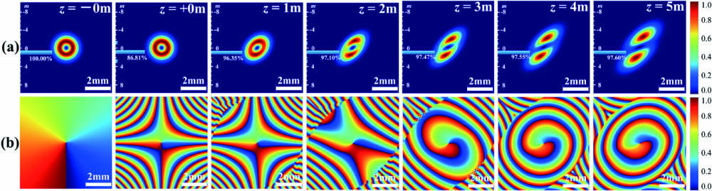
Fig. 1. Simulated propagation of the HGOV from 0 m to 5 m. z=−0m denotes the original OV with no CP at 0 m, and z=+0m denotes the OV immediately with the CP. (a) Simulated intensity distributions of the HGOV, where blue histograms denote the OAM spectra, and the percentage marked in the figures represents the proportion of m=1. (b) Simulated phase distributions corresponding to (a).

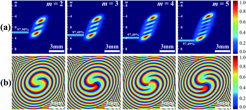
Fig. 2. Function of the self-measurement of the HGOV at the far-field. (a) Simulated intensity distributions of the HGOV of m=2, 3, 4, and 5, respectively, where blue histograms denote the OAM spectra, and the percentage marked in the figures represents the proportion of m=2, 3, 4, and 5, respectively. (b) Simulated phase distributions corresponding to (a).

Fig. 3. Self-sign-measurement of the HGOV. (a) Simulated intensity distributions of the HGOV of m=5, −5, where blue histograms denote the OAM spectra, and the percentage marked in the figures represents the proportion. (b) Simulated phase distributions corresponding to (a).

Fig. 4. Simulated distributions of HGOVs with different u′: u′=0.5u, 1.0u, 1.5u, and 2.0u, respectively. (a) Simulated intensity distributions, where blue histograms denote the OAM spectra, and the percentage marked in the figures represents the proportion of m=−5. (b) Simulated phase distributions corresponding to (a), where the white crosses mark the locations of the singularities.

Fig. 5. Simulated results of HGOVs of m=5 at 0°, 45°, 90°, and 135°, respectively. (a) Simulated intensity distributions. The white dotted lines are the axis of symmetry of HGOVs. (b) Simulated phase distributions corresponding to (a), where the white crosses mark the locations of the singularities.