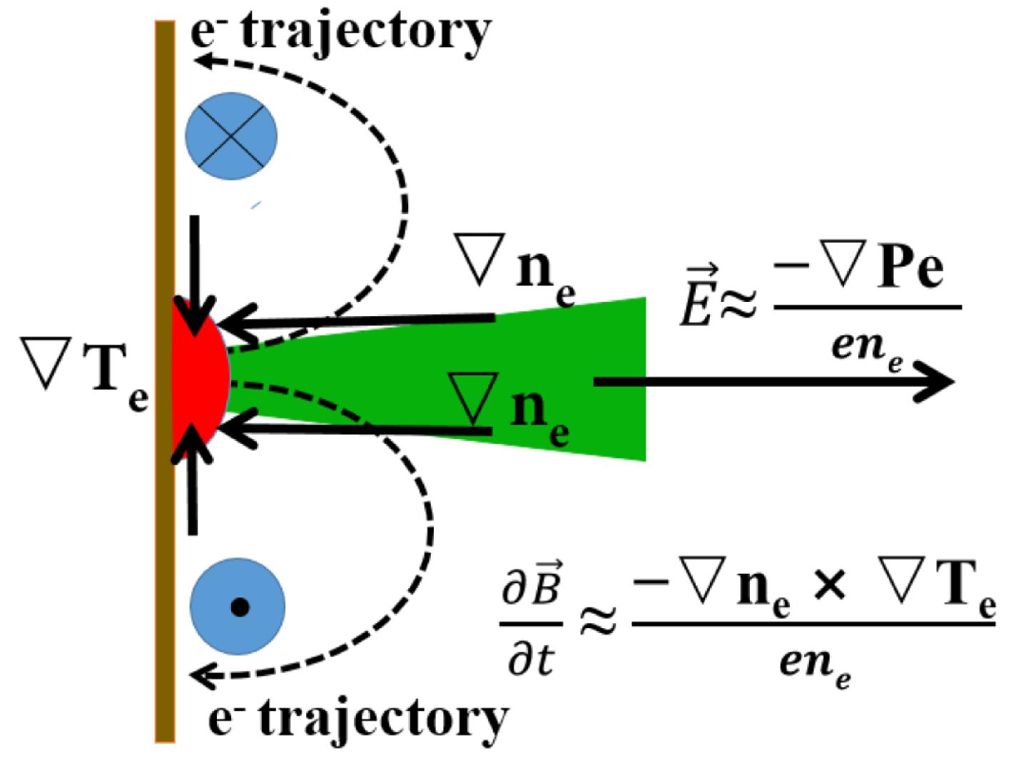
Fig. 1. Schematic diagram of the annular magnetic field in the plasma.

Fig. 2. The simulation of 2D particle-in-cell code, OSIRIS, showing hole-boring effects and regions of magnetic field. Region A represents the non-parallel temperature and density gradients; region B represents the ponderomotive source; region C represents the magnetic fields due to Weibel-like instability from laser-generated electron beams^[20].

Fig. 3. The capacitor-coil target. (a) Non-thermal hot electron is generated on the target surface of the capacitor coil. (b) The potential difference between the two capacitor coils is developed. (c) Loop current is generated in the coil.

Fig. 4. A schematic view of the MRX setup^[24].

Fig. 5. The contours of the out-of-plane quadrupole field in the diffusion region during reconnection^[4].

Fig. 6. A schematic view of VTF experimental setup^[28].

Fig. 7. Measured contour of the plasma density and the reconnection rate^[28].

Fig. 8. (a) Shadow image taken at a delay of 10 ns. (b) The electrons distribution around the coils at a delay of 3 ns^[35].

Fig. 9. Frontside copper images from focal spot separation scans using the OMEGA EP laser. horizontal line-outs are superimposed^[41].

Fig. 10. Snapshots (at from to ) of magnetic fields . (a)–(c) Azimuthal magnetic fields and (d)–(f) out-of-plane magnetic fields produced by a single incident laser. (g)–(i) and (j)–(l) by two incident lasers^[43].

Fig. 11. Reconnection electric field (at ) (a), (c) at , and (b), (d) at . Contributions to the generalized Ohm’s law from Equation (5) along the -axis at for , where (green line), (blue line), (brown line), (red line), and (purple line)^[43].

Fig. 12. Probe beam images of (a), (b) aluminum targets and (c), (d) gold targets^[50].

Fig. 13. Proton radiography data, (a) four or (b) two laser beams were employed to ablate a CH foil^[13].

Fig. 14. (a)–(e) Proton radiographic images of the magnetic field evolution. (f)–(j) Results of simulated proton radiography at the corresponding times, with overlaid magnetic field lines^[53].

Fig. 15. (a) Schematic diagram of magnetic field distribution and reconnection of the loop-top X-ray source. (b), (c) X-ray images taken by the pinhole camera in front of the target.

Fig. 16. (a) Experimental setup of Zhong et al. (2016)^[54]. (b) Black: experimental electron spectrum. Blue: simulated electron spectrum.

Fig. 17. (a), (b) The experimental results, two solid ellipses in the left panels represent the laser-produced magnetic systems, the gray contours (shadow images) in the right panels describe the trajectories of the energetic electrons. (c), (d) The simulations results, a group of electrons moving in the EM field without or with guide field, respectively.

Fig. 18. Hard X-ray image of a coronal arcade observed by YOHKOH satellite^[2], and standard model of CME^[64].

Fig. 19. Schematic of the magnetic field interactions between solar wind and Earth’s magnetosphere^[69].

Fig. 20. Upper panel: experimental setup of Zhang et al.^[71]. Down panel: X-ray image of shots with magnet of different field strengths, (a) null, (b) 3000 G and (c) 4000 G. The magnetic field is expressed as solid lines.

Fig. 21. Upper panel: POLAR satellite trajectory through the reconnection region in the Earth’s magnetosphere. Lower panel: the detail observed data^[73].

Fig. 22. Measured magnetic field in the reconnection layer for (a) high density and (b) low density cases^[4].

Fig. 23. (a) The experimental electron spectra of OMEGA EP^[41], which were measured at the target rear by a 5-channel electron spectrometer. The left panel is shot with 100 ps pulse-to-pulse delay, and the right panel is shot with no pulse-to-pulse delay. The lines with different colors are measured with angles with respect to the rear target normal. (b) and (c) are PIC simulation results using code OSIRIS. (b) The theoretical temporal evolution of electron spectrum in the midplane region. (c) The temporal evolution of maximum reconnection electric field (), non-thermal electron energy () and magnetic potential energy ().

Fig. 24. The electron distributions in the phase space of (, ). From the left to right, the columns correspond to the time , , , and , respectively. Row A is for , row B is for and row C is for ^[97].

Fig. 25. Energy spectra for the electrons (a) in the entire simulation box and (b) in the reconnection region only for . The solid blue curves are for the two-laser case and the red for the one laser case. In (a) the red line has been multiplied by a factor of 2 to compare with the blue line with two lasers. In (b) the dashed lines indicate the power law of the spectrum, , with the black line for and the green line for ^[97].

Table 1. The similarity of solar flares and the experiment of Zhong et al.^[51], with , and .