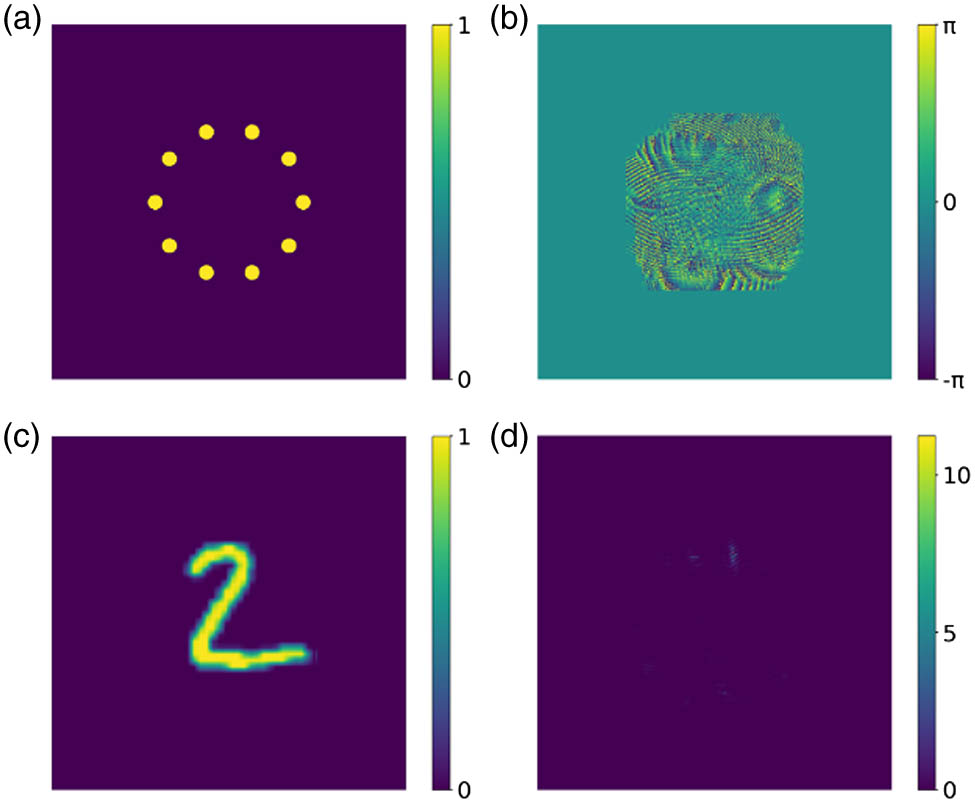
Fig. 1. Trained optical neural network (ONN). (a) The detector layer determines the location, where the light from the individual digits should be focused. The layout of the layer is a hyperparameter in our training. Here, each label corresponds to one bright circle (radius=100  μm) located 1 mm from the center of the image. The “0” label is on the positive x axis, and the rest of the labels are located sequentially counterclockwise on a circle. (b) Trained phase mask; (c) sample input image; (d) output of the neural network for the sample input shown in (c). For training, the neural network calculates the intensity at each label location and returns the highest-intensity label as its prediction. All images have dimensions of 600×600 pixels, which correspond to 4.8×4.8  mm.

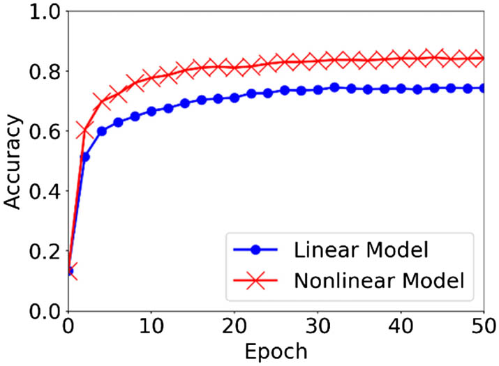
Fig. 2. Accuracy versus epoch for the linear model (blue dot) and the nonlinear model (red cross).

Fig. 3. Experimental setup. (a) Cartoon layout of the setup. The focal lengths of the lenses are: L1,50  mm; L2,300  mm; L3,150  mm; L4,150  mm; L5,100  mm. M indicates a flat mirror. (b) Photograph of the experiment.

Fig. 4. Nonlinear function showing the input–output curve for the incident intensity. The x axis is proportional to the input power, or the average pixel valve on the CCD camera without the vapor cell. The y axis is proportional to the output power, or the average pixel value on the CCD camera with the vapor cell in place. Inset, zoom-in plot showing the curve fit.

Table 1. Summary of ONN Accuracy in Percentage