Swept lasers are special tunable lasers whose wavelengths are tuned in a continuous or quasi-continuous mode and have been widely used in detection and sensing applications, such as spectroscopy [1], nondestructive testing [2], optical frequency domain reflectometry [3,4], and scanning source optical coherence tomography (SS-OCT) [5,6]. There is a large number of reports on the implementation so far, such as wavelength-swept amplified spontaneous emission sources [7], short cavity lasers [8,9], frequency modulated external cavity lasers [10,11], Fourier-domain mode-locked lasers [12,13], and swept vertical cavity surface-emitting lasers [14,15]. However, these lasers all require fast tunable filters, such as rotating diffraction gratings [16], polygonal mirrors [17], and tunable Fabry–Perot cavities [18,19], or require precise machining and design [20]. The mechanical structures in most tunable filters greatly limit the sweep speed, which reduces the performance of dynamic sensing in practical applications. In recent years, Takubo et al. demonstrated a dispersion-tuned swept-fiber laser (DTSFL) based on a dispersion tuning technique, which is an active mode-locking scheme with a large dispersion [21–23]. By changing the modulation frequency loaded on the intensity modulator, it can be swept rapidly without any optical filter. Different dispersive devices, gain media, and cavity structures were studied and compared, respectively, but the dynamic characteristics of the lasers were not investigated. The laser was optimized for OCT, and such fast-swept lasers have been successfully used for OCT imaging with a 250 kHz sweep rate [21]. Later, Riha et al. demonstrated a dual resonance akinetic optical swept source with an impressive sweep rate that can even reach MHz. The most important feature is that the sweep frequency is close to the fundamental resonant frequency of the cavity, which greatly improves the sweep rate of the DTSFL [24].

At present, the characterization of swept lasers mainly refers to their average or static characteristics, such as roll off performance or static instantaneous linewidth [25–27]. The research on time-resolved characteristics is mainly about intensity characteristics, which can be measured directly or analyzed theoretically [28]. Butler et al. demonstrated a self-delayed interferometric technique, which simultaneously measured the intensity and phase of single longitudinal mode and few longitudinal mode commercial swept lasers and reconstructed the complex electric field [29,30]. The technique revealed the internal modal dynamics of swept lasers and realized the research on their instantaneous characteristics. This method used an unbalanced interferometer based on a 3×3 coupler to measure the phase. It is difficult to be used in the research of multi-longitudinal mode swept lasers due to the limitation of the detector bandwidth. Hasegawa et al. proposed two models to analyze the steady-state characteristics of DTSFL without wavelength sweeping, but the dynamic behavior of its sweeping mode and laser build-up process has not been reported in detail [31].

Currently, the study of mode-locked lasers for dynamics using the time-stretching dispersive Fourier transform (TS-DFT) technique has been widely reported. Mapping spectral information into the time domain allows real-time observation of complex motions and interactions within the laser. This technique has become an excellent method for exploring laser dynamics and is particularly powerful in revealing the dynamics of unstable lasers [32–37]. In this paper, we learned from the advantages of the TS-DFT technology for rapid monitoring of laser behavior; measured the intensity dynamics of the DTSFL during startup, wavelength switching, and continuous wavelength sweeping; and calibrated the spectral information in real time using the relationship between modulation frequency and central wavelength, which was verified using numerical simulations. The results revealed the complex behavior of the DTSFL during operation for the first time, providing a new research basis for the practical application of such lasers.

The principle of dispersion tuning is to add a large dispersion element and an intensity modulator in the laser cavity to achieve active mode-locking through intensity modulation. For Nth-order mode-locking, the free spectral range (FSR) can be expressed as FSRN=fm=Ncn(λ)L,(1)where fm is the modulation frequency, c is the speed of light in the vacuum, L is the length of the laser cavity, n is the refractive index, and the FSR is a function of the wavelength λ. Therefore, when the fm is changed, the laser is mode-locked at different wavelengths to satisfy the resonance condition. The change of the central wavelength Δλ can be expressed as Δλ=−n0LcDtotalf0Δfm,(2)where f0 is the center of the modulation frequency; n0 is the refractive index at f0; the total dispersion is denoted by Dtotal; and Δfm is the variation of the modulation frequency. This equation shows that the central wavelength can vary linearly with fm [38].

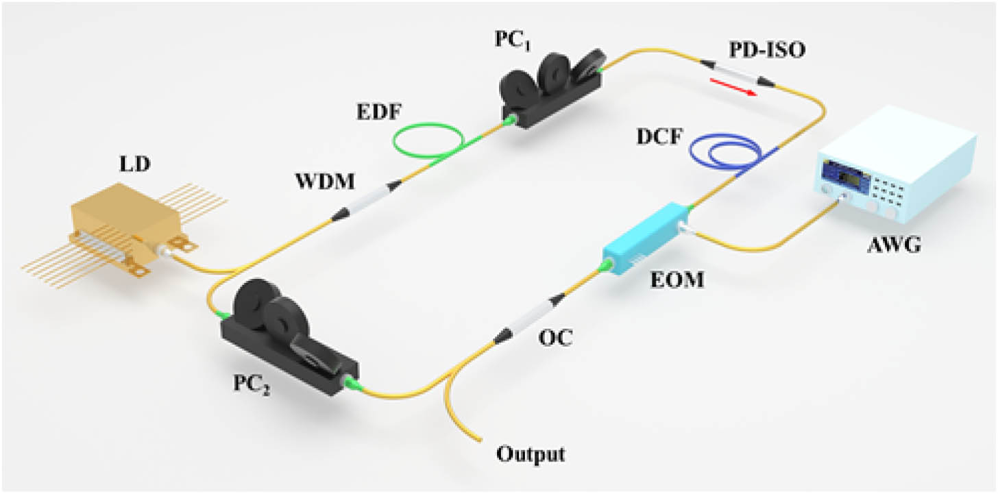
The setup of the swept laser is shown in Fig. 1. A 3-m erbium-doped fiber (Liekki, ER110) is pumped by a 980-nm-laser diode (Connet Ltd.) via wavelength division multiplexers (Flyin Ltd.). A ring fiber laser cavity is formed using a polarization-dependent isolator (Flyin Ltd.), an optical coupler (Flyin Ltd.) with a splitting ratio of 90:10, two polarization controllers, and a 150-m dispersion compensated fiber (DCF, G.655C/250). In order to realize active mode-locking, an electro-optical modulator (EOM, JDS Uniphase) driven by an arbitrary waveform generator (AWG, Tektronix AFG3102) is added to the ring cavity for intensity modulation. The other passive fibers are single-mode fibers (SMFs), and the total laser cavity length is ∼173m, corresponding to a laser fundamental frequency of ∼1.187MHz. The laser spectrum is measured by an optical spectrum analyzer (Yokogawa, AQ6370D) with a resolution of 0.02 nm. To demonstrate the dynamic characteristics of the swept laser, the laser output is detected by a photodetector (CETC, GD45220R) with an 18 GHz bandwidth, and then the electrical signal is measured by a high-speed real-time oscilloscope (Tektronix, DSA72004b) with a sampling rate of 25 GS/s.

In the experiment, the pump power of the laser diode (LD) was set to 200 mW. A sinusoidal signal generated by AWG with modulation frequency (fm) was loaded to the EOM. The laser source can output a narrow-band laser with the center wavelength varying at different modulation frequencies, and Fig. 2(a) shows the static laser spectra when the fm was tuned step by step. The laser wavelength varies from 1544.21 nm (λmin) to 1549.51 nm (λmax) when the fm was tuned from 198.252 MHz to 198.292 MHz. The 3 dB linewidth at different laser wavelengths varies slightly from 0.10 nm to 0.12 nm. Figure 2(b) shows the average spectra of the swept laser when the fm linearly swept from 198.252 MHz to 198.292 MHz in both positive sweep (PS) and negative sweep (NS) directions. The sweep duration in both the PS and the NS directions is 3 ms. It is worth noting that the swept wavelength range of the spectra is equal to the range of the static tuning, i.e., 5.3 nm. After that, the sinusoidal signal was switched between 198.252 MHz and 198.292 MHz with a rate of 250 Hz. Figure 2(c) shows the switched laser spectra. Due to the high speed of the switching, the captured spectrum is also an average result, where new wavelengths are clearly generated on both sides of λmin and λmax compared to Fig. 2(a). Generally speaking, the wavelength sweep range is limited by the peak gain region of the erbium-doped fiber (EDF) and competition from other oscillation modes. It is worth noting that the wavelength sweep range is also dependent on the state of polarization in the laser cavity. The maximum wavelength sweep range can be extended to 12 nm in our experiment. However, at the edge of the maximum sweep range, the laser becomes unstable due to low gain. We have obtained a stable output in the sweep range of 5.3 nm to facilitate the exploration of the intensity dynamics of the swept laser. We measured the power at the 10% port of the optical coupler (OC). The output power was ∼280μW in static mode and ∼260μW in switching mode and sweeping mode. In addition, the output power and sweep range within 2 h at intervals of 10 min were measured. The results are shown in Fig. 2(d). The laser can maintain excellent stability in long-term operation. In order to further investigate the specific behavior of this laser during the wavelength switching mode and continuous sweeping mode, we used the TS-DFT technique to record signals, which is widely used in studying soliton dynamics [39–41]. In the TS-DFT technique, a long DCF is usually added after the laser output to stretch the laser pulse in time domain. In our experiment, owing to the long DCF in the cavity, the output laser itself has a large chirp itself. Hence, the oscilloscope can record a suitable pulse signal even without using an additional dispersive fiber to stretch the output laser in the time domain. In fact, a comparison with the signal after the additional 4 km DCF shows that it is almost indistinguishable from the original signal, but the optical amplifier added to compensate for the power loss increases the background noise and makes the system more complex.

First, we investigated the dynamical characteristics of the switching mode. The intensity dynamics process corresponding to Fig. 2(c) was measured. Figure 3(a) shows the results of the time and intensity changing with round trips (RTs). The repetition rate of the laser stays the same with the fm due to the intensity modulation of the EOM, i.e., 168 pulses are output in one RT. To make the image more intuitive, the time of a single RT is set to be about 168/198.292 μs so that the pulses with a repetition rate of 198.292 MHz are shown in Fig. 3(a) as a nearly horizontal straight beam, while the pulse beam with a repetition rate of 198.252 MHz exhibits a downward sloping trend. Integrating the energy within each RT in Fig. 3(a) to obtain the blue curve in Fig. 3(b), it can be seen that the energy first decays rapidly and then increases sharply at the beginning of the switching mode. This process (stage 1, RT≈1210–2120; stage 3, RT≈3600–4510) is similar to the relaxation oscillation (RO) at the early stage of soliton establishment [42]. The difference is that since the pump power is kept constant in the experiment and the EOM is constantly intensity modulated, this RO process shows a very smooth damped oscillation in energy, and the oscillation stabilizes after about 910 RTs and the laser starts to operate stably (stage 2, RT≈2120–3600; stage 4, RT≈4510–5990). Figure 3(c) shows an enlarged view of the yellow dashed box in Fig. 3(a), which clearly indicates the pulse evolution before and after the fm switching. Interestingly, the spacing of the energy peaks decreases during the oscillation, and a partial close-up is shown in Fig. 3(d), where the red circles represent the peak positions. The energy in the cavity at the beginning of the RO is much larger than that in the steady state. The very high energy excites the nonlinear effect in the cavity, which is mainly shown as a spectral broadening caused by the four-wave mixing effect. That is why new wavelengths other than λmin and λmax are generated during the switching mode in Fig. 2(c), but we cannot further investigate the generation and disappearance of wavelengths during the process due to the limitation of the detector.

After that, the sinusoidal signal was fixed at fm=198.292MHz for 1 ms, then was swept to 198.252 MHz within 2 ms, and back to 198.292 MHz within 2 ms. The above process is repeated continuously. Figure 4(a) shows the partial intensity dynamics of this periodic modulation process. Since the cavity time of each RT is slightly different due to the constant change of the fm, while the time period in Fig. 4(a) remains fixed, the pulse curve during the sweep bends and changes with the increase of RTs, and Fig. 4(b) shows the corresponding energy integration curve. Figure 4(c) shows the enlarged view of the yellow dashed box in Fig. 4(a), which clearly demonstrates the process before and after static mode. The whole process contains three typical stages. In the first stage with RTs from ∼1200 to ∼2400, the laser transits from the last sweep mode to the static mode. At the beginning of this state, pulses remaining in the sweep mode begin to gradually decay due to the EOM starting to intervene again to control the repetition rate of the pulses, forming 168 pulses with uniform intervals together with the growing background pulses at the same time. The pulses return to a steady state after ∼700 RTs, and the laser starts to return to relatively stable operation.

In the second stage with RTs from 2400 to 3100, the laser is changed from the static mode to the next sweeping mode. In the start-up process of the sweeping mode, the energy integration curve also exhibits RO. This phenomenon is similar to that in the switching mode, as discussed in Fig. 3. The difference is that the smoothness of the energy integration curve decreases significantly because the fm is constantly changing in the sweeping mode. In addition, the EOM seems to lose its modulation effect on the laser in RO, resulting in lots of pulses fixed in the static mode fading into the background due to gain competition. Consequently, the few pulses with higher initial energy keep gaining amplification, while the rest of the pulses keep decaying in the competition and finally vanish completely at the end of RO. The energy of the remaining pulse reaches its maximum at this point. The wavelengths and energy are also different when the laser enters the steady mode, showing randomness and making the different cycles not memorable and correlated [33]. This is mainly due to different initial energy of each pulse during gain competition, which shows a selective amplification process. The duration of the gain competition is also slightly different in each cycle, resulting in different center wavelengths and energy when the laser enters the steady state.

In the third stage with RTs from 3100 to 7200, the laser successively sweeps in the NS and PS directions. The energy in the laser cavity remains stable, which indicates that the laser can keep sweeping in a stable state after the end of RO. As long as the fm changes continuously without going through the static mode, the remaining pulses can always exist stably, not only keeping the number constant, but also maintaining a fixed time interval. Even if there is an environmental disturbance, the stability is not affected in the time domain. Figure 4(d) shows a close-up of the energy integration curve near RT = 5330, and the red circles represent the data points. The energy has been oscillating periodically during the sweeping mode. This is due to the fact that the central wavelength is constantly changing during the sweep, and this process makes the spectrum have a tendency to constantly broaden. Because the sweeping speed is extremely fast and the pump power remains constant, the spectrum is constantly broadened and compressed within a very small range due to the clamping of the total energy, which shows periodic oscillations in energy.

After removing the static process, the sinusoidal signal was first linearly swept from 198.146 MHz to 198.252 MHz in the NS direction and then back to 198.146 MHz in the PS direction. The durations of the NS and PS sweeping are 1 ms and 2 ms, respectively. Figure 5(a) shows the intensity dynamics of this periodic modulation process, and Fig. 5(b) shows the corresponding energy integration curve. The lowest energy occurs at the turning points of the sweep direction, i.e., fm=198.252MHz and 198.146 MHz corresponding to points 1 and 3 in Fig. 5(a). The highest energy occurs at the middle position, i.e., fm=192.272MHz corresponding to points 2 and 4 in Fig. 5(a). This is because at different polarization states, the central wavelength and sweep range of the swept laser are different, but the corresponding gain spectrum is always a parabolic curve with the center of the sweep range as the vertex. In addition, the independent energy integration of the upper and lower pulses in Fig. 5(a) is obtained in Figs. 5(c) and 5(d), respectively. Since the total energy in the laser cavity is certain, the energy in each pulse shows a mutually supplementary trend, indicating that there is energy exchange between the pulses. Since the stable operation of the laser in the continuous sweep mode does not generate new wavelengths, the modulation frequency can linearly correspond to the central wavelength [21]. By deriving the pulse curve in Fig. 5(a), the periodic curve shown in Fig. 6(a) can be obtained, which clearly shows the linear variation of the central wavelengths and the fm with the RTs. Since the difference between the instantaneous linewidth of the spectrum at the static mode and sweeping mode is small [31], the spectral linewidth at the sweeping mode is expressed in terms of relative wavelengths according to the linewidth at the static mode. The pulse curve at the bottom of Fig. 5(a) is “straightened” to obtain Fig. 6(b) (the spectral resolution of the time stretch is 0.01 nm from the experimental results), which clearly shows that the pulse width (i.e., the linewidth of the spectra) of the laser varies periodically over a range during the sweeping mode, confirming the conclusion that the spectra are continuously broadened and compressed within a very small range. In our laser cavity with normal dispersion, we did not observe obvious linewidth change in two sweep directions, which is consistent with the simulation [31].

From the above conclusion, it can be seen that the center wavelength of the laser gradually approaches and is swept to 1546.59 nm during RT=3321−3341, the short-time Fourier transform of the time-domain signal is done at RT = 3321, 3331, and 3341, and a close-up of the same center frequency obtains the spectrum shown in Fig. 7, revealing the variation of the multi-longitudinal mode of the laser in the process. In the whole process, the laser is composed of multiple longitudinal modes, and the central frequency of the spectrum keeps varying with time, and the intensity distribution of the frequencies does not seem to be correlated, so it cannot show a stable soliton form in the time domain. However, the frequency interval between the longitudinal modes remains fixed and is the same as the fundamental frequency of the laser cavity, which is 1.187 MHz. This also further indicates that the intensity modulation of the EOM in this state nearly disappears. As the central wavelength gradually approaches 1546.59 nm, the intensity of each longitudinal mode gradually increases and finally reaches the maximum at the central wavelength, after which it gradually returns to the low-energy state and finally disappears in the background noise.

To verify the conclusions mentioned above, a simplified cavity model is used to numerically simulate and illustrate the laser generation and sweeping process, as shown in Fig. 8. It consists of a 3-m EDF, a 150-m DCF, an EOM, and two PCs. The transmission matrix method is employed to describe the change of the electric field distribution when the light passes through each component. The Ginzburg–Landau equation was used to track the evolution of the electric field in the cavity, ∂A∂z−iβ22∂2A∂t2−iγ|A|2A=(g−α)A2+g2Ωg2∂2A∂t2,(3)where A is the slowly varying amplitude electric field, t and z represent the transmission time and distance, β2 and γ are the second-order dispersion and the third-order nonlinear coefficient, g is the saturation gain of the fiber, α is the attenuation, Ωg is the laser gain bandwidth in the passive fiber, and g=0 in the EDF, g(z,t)=g(z)=g0(1+1Es∫0twin|A(z,t)|2dt)−1,(4)where g0 is the small signal gain factor, Es is the gain saturation energy, and twin is the size of the simulation window.

Compared to the theoretical model in Ref. [31], it is worth noting that we ignore the modulation term in Eq. (3). In fact, we found that the EOM actually loses its modulation effect during the sweeping mode in the experiments. It makes no difference whether the center of the modulation frequency is set to the fundamental frequency of the laser or to an integer multiple of the fundamental frequency. Therefore, the theoretical model can be simplified to a passively mode-locked laser. The EOM is in fact equivalent to an optical time-delay line [43]. The change in fm can be replaced by a change in the cavity length, which not only greatly simplifies the calculation but also gives the same results.

In our experiment, the spectral linewidth of the laser can be adjusted by changing the state of the polarization in the cavity. In order to consider the influence of the polarization, the light propagation in the passive fiber is described by the two coupled nonlinear Schrödinger equations, $$\begin{gathered} ∂Ax∂z−iβ22∂2Ax∂t2−iγ(|Ax|2A+23|Ay|2)Ax−i3γAx*Ay2=0, \\ ∂Ay∂z−iβ22∂2Ay∂t2−iγ(|Ay|2A+23|Ax|2)Ay−i3γAy*Ax2=0, \end{gathered}$$(5)where Ax and Ay are the field amplitudes of two orthogonal polarization components.

Based on the above theory, we simulated the switching mode and static-sweeping mode by picking 213 sampling points. The laser parameters are consistent with the experiment, as specified in Table 1. The total linear loss of the laser is 30% (including component insertion loss, fiber splicing loss, and bending loss). The spectral and pulse evolutions of the switching mode are shown in Figs. 9(a) and 9(b), respectively. At RT=500, the center wavelength of the laser with a 3 dB linewidth of 0.07 nm is switched from 1548.2 nm to 1551.8 nm, and then returns back at RT=1000. Similar to the experimental results, the laser energy decays sharply at the beginning of the switching mode, and then gradually returns to a stable state. During the process, the spectrum is significantly broadened, and the magnitude of the broadening and the recovery time are related to the value of the gain. Figures 9(c) and 9(d) show the spectral and pulse evolutions of the laser in the sweeping mode, respectively. Starting from RT=350, the center wavelength of the laser is swept between 1550 nm and 1548.5 nm with a single sweep period of 400 RTs. At RT=350, the laser also decays in energy when it enters the sweeping mode from the static mode, but the laser keeps operating stably during the sweeping mode after restoring stability, and there is no spectral broadening during the process. Although there are inflection points in the spectrum at RT=750 and 1150 due to the change in sweeping direction, these do not affect the stability of the laser in the time domain due to the low intensity at the points. In addition, there is no significant broadening of the 3 dB linewidth of the spectrum in the sweeping mode compared to the static mode, which provides the theoretical basis for Fig. 6. The model also predicts the maximum sweep speed of the laser, and the simulation results show that when the sweep range, gain, and center wavelength are determined, the faster the sweep speed is, the worse the stability of the laser is. The sweep speed exceeds the threshold, and the laser will enter the intermediate state of the sweeping mode and the static mode. In the above settings, the maximum sweep speed of the laser can theoretically exceed 30 kHz.Table 1.

Parameters Used in Simulation

All parameters in the simulation are consistent with the experiment. Except for the parameters mentioned above, all other parameters are listed in Table 1.

In this paper, we characterized the dynamics of the DTSFL by using a high-speed oscilloscope. The wavelength of the DTSFL was linearly swept by continuously changing the modulation frequency of the EOM in the laser cavity. Since the large dispersion in the cavity makes the laser generate a chirped laser directly, the intensity dynamics during the switching mode, the static-sweeping mode, and the continuous sweeping mode are measured using a high-speed oscilloscope, respectively. It has been shown that if the fm changes discontinuously, then the laser generates RO, and the nonlinear effect caused by the high energy makes the laser generate new wavelengths, which is not beneficial for the application of swept lasers. If the fm changes continuously, then the modulation effect of the EOM is weakened, and the laser outputs a random number and position of pulses in one RT. The real-time wavelength calibration of the swept laser is achieved by the correspondence between the fm and the central wavelength in the continuously sweeping mode. The results of the numerical simulation are consistent with the experimental results. These results clearly show the dynamic behavior of the swept laser at different modulation modes. Excluding severe environmental disturbances and ensuring continuous sweeping of the fm is the key to the stable operation of the laser, and the laser has good symmetry in the PS and NS stages. These findings provide a theoretical basis for the application of such lasers in the future.