
Yutian Wang, Songnian Fu, Jian Kong, Andrey Komarov, Mariusz Klimczak, Ryszard Buczyński, Xiahui Tang, Ming Tang, Yuwen Qin, Luming Zhao. Nonlinear Fourier transform enabled eigenvalue spectrum investigation for fiber laser radiation[J]. Photonics Research, 2021, 9(8): 1531
- Photonics Research
- Vol. 9, Issue 8, 1531 (2021)
Abstract
1. INTRODUCTION
In steady-state operation, mode-locked lasers can generate highly stable pulse trains, which have various applications in science and engineering [1,2]. From the applications perspective, the ultrafast fiber laser offers its inherent advantages of robust operation and compact footprint [3,4]. Beyond its very evident practical importance, ultrafast fiber lasers are also interesting from the standpoint of physics as a platform for investigating various aspects of nonlinear wave dynamics [5–7]. Getting a considerable insight into the nonlinear dynamics and instabilities of fiber lasers is promising for discovering new operation regimes with potentially superior characteristics [8]. In contrast to a light pulse propagation over a fiber—where the system is conservative with the assumption of lossless propagation—a fiber laser is a paradigm of dissipative systems, where gain and loss affect the pulse generation, while simultaneously it is a periodic boundary system. Due to these dynamical changes, nonstationary pulses cannot be efficiently represented by the use of a linear combination of stationary signals. Therefore, traditional Fourier transform is not always suitable for investigation of fiber laser radiation. To solve this technological hurdle, several advanced characterization methodologies have been demonstrated, providing new ultrafast measurement tools to reveal transient phenomena arising in nonlinear laser dynamics. For instance, the dispersive Fourier transform (DFT) method has been successfully applied in fiber lasers for investigating soliton explosions [9], bound solitons [10,11], transition dynamics from -switching to mode locking [12], and buildup dynamics of harmonic mode locking [13]. Furthermore, the methodology of space–time duality has been successfully exploited to realize time lenses for direct observation of rogue waves [14] and unknown soliton dynamics [15]. It is now well known that, when solitons are generated in fiber lasers, there appear sidebands on the spectrum, such as Kelly sidebands [16] and other incoherent sidebands [17]. The incoherent sidebands can be removed by reducing pump power or intracavity polarization modulation, while the coherent sidebands such as Kelly sidebands always exist. Kelly sidebands could be considered as one of the resonant continuous wave (CW) backgrounds [18]. Although the DFT and time lens methods have successfully realized laser output monitoring in real time, the dynamics of solitons alone or of a pure soliton in a cavity is still unclear.
Recently, an elegant method of nonlinear Fourier transform (NFT) has attained attraction in the ultrafast optics community [19]. It is a powerful mathematical tool, which enables solving problems of wave propagation in some nonlinear media, especially in the field of soliton theory. Also known as inverse scattering transform, the NFT can decompose the signal into a continuous spectrum (nonsoliton components) and a discrete spectrum (soliton components) to obtain the corresponding nonlinear spectrum [20]. With the help of such an approach, information can be encoded into the nonlinear spectrum of the signal, which can effectively address the nonlinear transmission impairments arising in standard single-mode fiber (SMF) transmission [21,22]. Meanwhile, as a method to obtain analytic solutions to the nonlinear Schrödinger equation (NLSE), the NFT can be used to analyze signals in optical fibers, such as rogue waves [23] and Kerr optical frequency combs [24]. In particular, such NFT methodology provides a viewpoint on the new physics of laser dynamics. Specifically, the NFT has been shown to have the capability to characterize the ultrashort pulse in the nonlinear frequency domain [25–27]. Based on the NFT, we have proposed a method of soliton distillation to distinguish solitons from the resonant CW background according to their different eigenvalue distributions [28].
Fiber lasers operated in steady states can be classified into the state of single pulse, the state of period doubling of single pulse, the states of dual pulses either tightly bound or loosely distributed, the states of three pulses, and various combinations of the above-mentioned states. Since fiber lasers are a paradigm of dissipative systems, all the pulses sustained with the CW background. It is interesting to understand the performance of soliton alone in a fiber laser. As the CW always functions as an energy buffer, it is fundamental to get insight into soliton interaction without the CW. Therefore, we can use the approach of NFT-based soliton distillation to separate solitons from the CW background. We noted that we applied the NFT to deal with signal output from the fiber laser, not the one inside the fiber laser cavity.
Sign up for Photonics Research TOC. Get the latest issue of Photonics Research delivered right to you!Sign up now
In the following section, we report on the dynamics of various stable states arising in a fiber laser after the NFT is applied, including the state of single pulse, the state of single pulse in period doubling, and the states of double pulses and triple pulses. Furthermore, by using the approach of soliton distillation, we recover the pure solitons of those pulses. It is verified that the CW background indeed buffers solitons and affects the performance of coexisting solitons. The results provide a unique insight of the internal evolution of pure solitons without the CW background influence.
2. RESULTS AND DISCUSSIONS
The details of NFT processing can be found in Appendix A. A typical output of the passively mode-locked fiber laser and its optical spectrum are shown in Figs. 1(a) and 1(b). Different from theoretical soliton, there is a pedestal arising in the temporal profile and Kelly sidebands symmetrically exist in its optical spectrum. The eigenvalues distribution is shown in Fig. 1(c). The eigenvalue corresponding to the soliton has large imaginary parts and almost zero real parts, which indicates that the soliton has a near-zero velocity. The imaginary part of the soliton eigenvalue is only determined by the amplitude of the pulse. Meanwhile, distinctly from the eigenvalue distribution of a theoretical soliton, some eigenvalues have nonzero real parts and relatively small imaginary parts, indicative of nonzero velocities of the corresponding temporal features of the resonant CW background. The real parts of CW eigenvalues are related to its frequency.
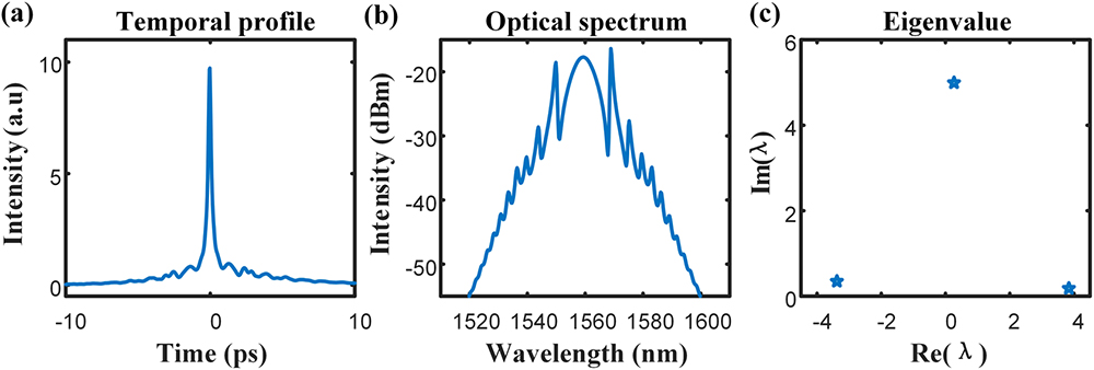
Figure 1.(a) Temporal profile, (b) optical spectrum, and (c) eigenvalues of a pulse from the fiber laser.
Obviously, the eigenvalues of the pulse from the fiber laser are different from that of a theoretical soliton, which is attributed to the coexisting resonant CW background. Since the soliton and the resonant CW background have different eigenvalue distributions, it is feasible to separate a pure soliton from the resonant CW background based on the NFT. Then, we select the eigenvalue corresponding to the soliton and reconstruct the temporal waveform by the inverse NFT (INFT) [28]. The temporal profile, optical spectrum, and eigenvalue distribution of filtered soliton are shown in Fig. 2. There is a reduction of the optical spectrum due to the taking-away of resonant CW background.
![]()
Figure 2.(a) Temporal profile, (b) optical spectrum, and (c) eigenvalue of the filtered soliton.
Then, we analyze the starting dynamics of solitons in terms of the eigenvalue spectrum. Figure 3 shows the starting dynamics of the fiber laser. Starting from a small signal, the intensity evolution to a stable pulse is shown in Fig. 3(a), where different colors indicate different intensities. Figure 3(b) shows the evolution of eigenvalues versus round trips in 3D format, where the axis is the real part, the axis is the round trip, and the axis is the imaginary part. During the soliton generation, there exist some eigenvalues with small imaginary parts in the nonlinear spectrum, corresponding to the resonant CW background. Then, the intensity evolution and eigenvalue evolution of the filtered soliton are shown in Figs. 3(c) and 3(d), respectively. After soliton distillation [28], we successfully obtained the soliton component of the generated pulse, i.e., the pure soliton.
![]()
Figure 3.NFT data evolution obtained from the measurement of the fiber laser: (a) real-time spatial–temporal dynamics of laser evolution from full-field measurements; (b) evolution of the eigenvalues; (c) dynamics of filtered soliton evolution; and (d) evolution of its eigenvalues.
When the pump power is increased to beyond a threshold, the pulse starts to periodically oscillate and return to itself every two round trips, which is called period doubling [29]. The dynamics of pulses in period doubling is shown in Fig. 4. The intensity of the pulse shuttles periodically between two states, as shown in Fig. 4(a). Figures 4(b) and 4(c) show the pulse temporal width and the imaginary part evolution of the eigenvalue, respectively. Synchronously, the pulse temporal width and eigenvalue oscillate with the same period of pulse intensity. The intensity variation of the optical field is accompanied by a variation of eigenvalue spatial distribution. Such a relationship between the eigenvalue spectrum and the emergent features in the spatial–temporal dynamics demonstrates the effectiveness of the NFT formalism in revealing the underlying solitary modes embedded into the laser output. After soliton distillation, the intensity evolution of the filtered soliton is shown in Fig. 4(d). Distinctly from the stable pulse in Fig. 3, the pulses in period doubling have different eigenvalue distributions. This is because the imaginary part of the eigenvalue is related to the pulse intensity. Therefore, the change of eigenvalue imaginary part can reflect the periodic variation of pulse intensity as expected.
![]()
Figure 4.NFT data evolution obtained from the output of the fiber laser in period doubling: (a) real-time spatial–temporal dynamics of laser evolution from full-field measurements; (b) the temporal width of the pulse during every round trip; (c) the evolution of the imaginary parts of eigenvalues; and (d) the evolution of filtered soliton evolution.
The temporal profiles and optical spectra of the two different states of pulses in period doubling are shown in Fig. 5. The pulse in state 1 has lower intensity and its temporal width is about 190 fs. Meanwhile, the pulse in state 2 has higher intensity and its temporal width is about 160 fs. After soliton distillation, the temporal profiles and optical spectra of the two different states of pure soliton are also shown in Fig. 5. The soliton in state 1 has relatively lower intensity and a narrower spectral bandwidth of , while the soliton in state 2 has higher intensity and wider spectral bandwidth of , which are qualitatively similar to the pulse.
![]()
Figure 5.Temporal profiles and optical spectra of the period doubling pulse without and with soliton distillation: (a), (b) state 1; (c), (d) state 2.
Under appropriate parameter setting and operation conditions, typical emergence of multi-pulse states consisting of more than one pulse can be easily obtained from the fiber laser. Tightly bound solitons can be referred as soliton molecules if there exists strong soliton interaction [30]. Depending on the pulse separation and pulse intensity, the double pulse states can be classified into unstable and stable states, respectively. Setting the initial condition of the fiber laser as , the initial pulse can develop into unstable double pulses. The dynamic process of double pulses under unstable evolution can be obtained, as shown in Figs. 6(a)–6(d). The intensity evolution of the pulse is shown in Fig. 6(a), where different colors correspond to different intensities. During the evolution, the initial pulse splits into two pulses and their amplitudes sharply increase. After 60 round trips, the unstable double pulses are generated and there is an energy exchange between the two pulses, accompanied by the variation of their intensities. Figure 6(b) shows the imaginary part evolution of eigenvalues with respect to the round trip. Clearly, there are two eigenvalues, and each eigenvalue is associated with a pulse. Two eigenvalues first keep increasing and then increase and decrease alternately, revealing the energy exchange between the two pulses. After the soliton distillation, the temporal profiles of filtered soliton pairs are shown in Fig. 6(d). It is found that the soliton separation always reduced after the soliton distillation.
![]()
Figure 6.NFT data evolution obtained from the double pulses under (a)–(d) unstable and (e)–(l) stable state: (a), (e), (i) real-time spatial–temporal dynamics of laser evolution from full-field measurements; (b), (f), (j) the evolution of the imaginary parts of eigenvalues; (c), (g), (k) the temporal profiles without soliton distillation; (d), (h), (l) the temporal profiles with soliton distillation.
Changing the initial condition of the fiber laser as , stable double pulses can be observed with appropriate parameter setting. Figure 6(e) shows the stable evolution of two pulses. However, it is difficult to distinguish whether there is energy exchange between the two pulses from Fig. 6(e) as their intensities are close to each other. During the evolution, there indeed exists a weak energy exchange between the two pulses, as shown in Fig. 6(f), when we monitored the stable evolution in terms of eigenvalues obtained from the NFT. The imaginary part evolution of eigenvalues with respect to the round trip clearly suggests the energy exchange. Therefore, the NFT method can disclose details during pulse evolution for the states of double pulses even when their pulse intensities are close.
Similar to the case of two unstable pulses, for the case of two stable pulses (identified by the pulse separation and pulse intensity), soliton separation reduces after distillation. Figures 6(g) and 6(h) show the temporal profiles of stable double pulses without and with soliton distillation, respectively. The intensity difference is shown in the zoom-in insets. It is verified that the CW background actually buffers solitons and affects the performance of the coexisting soliton pair.
We purposely changed the initial condition and achieved a state of two stable pulses with pulse separation of 26 ps, as shown in Figs. 6(i)–6(l). As the pulse separation is now much longer, the CW-based interaction between the two pulses should be weaker compared to the state shown in Figs. 6(e)–6(h), which is verified by the imaginary part evolution of eigenvalues as shown in Fig. 6(j). Now the imaginary part evolutions of eigenvalues of the two far-apart pulses are nearly overlapped entirely. Again, soliton separation reduces after distillation.
Adjusting the parameters in the laser cavity, the initial pulse can also evolve into unstable triple pulses. Figures 7(a)–7(d) show the splitting dynamic process of the initial pulse . First, the initial pulse splits into two pulses, accompanied by the third pulse with relatively low amplitude, as shown in Fig. 7(a). Figure 7(b) shows the imaginary part evolution of eigenvalues with respect to the round trip. An eigenvalue with an imaginary part of refers to the pulse with relatively low amplitude, around the first 50 round trips. Then, the unstable triple pulses are generated, and the eigenvalues increase and decrease alternately, revealing the energy exchange between the three pulses. Figures 7(c) and 7(d) show the temporal profiles of triple pulses with and without soliton distillation, respectively. Similar to double pulses, the pulse separation of triple pulses reduces. Alternatively, setting the initial condition of the fiber laser as , stable triple pulses can be easily obtained with appropriate parameter setting. Here is a variable, which is associated with pulse separation of the input pulse. When setting initial pulse separation , the dynamic process, eigenvalue evolution, temporal profiles, and filtered solitons of stable triple pulses are shown in Figs. 7(e)–7(h), respectively. Under stable operation, the pulse separation is relatively large. The inset in Fig. 7(f) shows the eigenvalues distributions of stable triple pulses. Their imaginary parts are approximately equal, revealing the triple-soliton pulses have approximately equal amplitudes in the time domain. Generally, the interaction between solitons is realized by the resonant and nonresonant CW background in the case of stable multi-pulses. As for stable triple pulses, in the nonlinear frequency domain, there are more eigenvalues with almost zero real parts on the bottom, due to the nonresonant CW background. After soliton distillation, soliton separation reduced significantly as both the resonant and nonresonant CW backgrounds are filtered out, as shown in Fig. 7(h).
![]()
Figure 7.NFT data evolution obtained from the triple pulses under (a)–(d) unstable and (e)–(h) stable state: (a), (e) real-time spatial–temporal dynamics of laser evolution from full-field measurements; (b), (f) the evolution of the imaginary parts of eigenvalues; (c), (g) the temporal profiles without soliton distillation; (d), (h) the temporal profiles with soliton distillation.
Generally, triple pulses have three pulse separations and we name them , , and , respectively, as shown in Fig. 8(a). Figures 8(b) and 8(c) show the pulse separation and purified soliton separation with different initial pulse separation setting of , respectively. Provided that , the pulse separation of the stable multiple pulse output from the fiber laser is always the same as the initial setting. When increases, the pulse separation accordingly increases. After soliton distillation, the soliton separation is greatly reduced. It is straightforward that soliton separation can be manipulated and much reduced if the CW background is fully removed, which paves a way for manipulating solitons without CW background and shows a new viewpoint on acquisition of pure solitons from a fiber laser for soliton communication. It is feasible to obtain multiple solitons with much closer separation by employing the soliton distillation scheme.
![]()
Figure 8.(a) Three pulse separations of triple pulses, (b) pulse separation, and (c) filtered soliton separation with different initial pulse separation
3. CONCLUSION
In summary, the eigenvalues of a pulse can be obtained by using the NFT, whose real and imaginary parts correspond to the frequency and amplitude of the pulse, respectively. Pure solitons can be separated from the CW background according to different eigenvalue distributions. It is feasible to obtain NFT results from real-time spatial–temporal dynamics of various laser pulsing evolutions, for instance, single pulse, single pulse in period doubling, double pulses, and triple pulses. It is found that the imaginary part of the eigenvalue evolution of single pulse is consistent with its intensity evolution. As for coexisting multiple pulses, the imaginary parts of their eigenvalues alternatively increase or decrease during the evolution, revealing the changes in their intensity due to the energy exchange between the pulses during evolution. The degree of overlapping between the different evolutions of the imaginary parts of their eigenvalue of different pulses in the states of multiple pulses can be used to identify the pulse intensity difference, which is more obvious comparing with pulse intensity evolutions. With the help of soliton distillation, we obtained pure solitons from those pulses. However, much closer soliton separation is always achieved. As a promising signal processing tool, the NFT paves a new way for investigating soliton interaction in nonlinear systems. Our results suggest that the NFT can be a featured characterization method in ultrafast optics. Recently, Vasylchenkova
APPENDIX A
Generally, the NFT is a method to solve the initial value problem for the nonlinear evolution equation. In an optical fiber, where the signal evolution occurs along the fiber, the initial condition corresponds to the time-domain waveform at the transmitter and its evolution satisfies the NLSE. With the assumption of a noiseless and lossless fiber, the NLSE is a well-known and practically important example of the following integrable equation [
As it is well known, the optical solitons are the balanced result of dispersion and nonlinearity, where they can propagate without distortion over the fiber. Similarly, for the pure NLSE, the complex eigenvalues also stay invariant during the pulse evolution. Therefore, by analyzing the nonlinear spectrum of the evolving signal, we can readily segregate the eigenvalue that refers to soliton components of the signal from the continuous spectrum. When calculating the nonlinear spectrum, different settings of normalization parameters may lead to different energy distributions between nonlinear spectral components [
Figure
![]()
Figure 9.Temporal profiles of (a)
![]()
Figure 10.(a) Passively mode-locked fiber laser. ISO, isolator; PC, polarization controller; WDM, wavelength-division multiplexer; OC, output coupler. (b) Corresponding digital signal processing (DSP) flows of coherent receiver.
Then, the NFT determined eigenvalue can be calculated from the full-field information of the pulse. An important step for obtaining the nonlinear frequency spectrum is the normalization of the input field, scaling the time and amplitude [
References
[1] P. M. W. French. The generation of ultrashort pulses. Rep. Prog. Phys., 58, 169-267(1995).
[2] U. Keller. Recent developments in compact ultrafast lasers. Nature, 424, 831-838(2003).
[3] A. Martinez, Z. P. Sun. Nanotube and graphene saturable absorbers for fiber lasers. Nat. Photonics, 7, 842-845(2013).
[4] U. Andral, R. S. Fodil, F. Amrani, F. Billard, E. Hertz, P. Grelu. Fiber laser mode locked through an evolutionary algorithm. Optica, 2, 275-278(2015).
[5] S. Kobtsev, S. Kukarin, S. Smirnov, S. K. Turitsyn, A. Latkin. Generation of double-scale femto/pico-second optical lumps in mode-locked fiber lasers. Opt. Express, 17, 20707-20713(2009).
[6] N. Tarasov, A. M. Perego, D. V. Churkin, K. Staliunas, S. K. Turitsyn. Mode-locking via dissipative Faraday instability. Nat. Commun., 7, 12441(2016).
[7] J. Xu, L. Huang, M. Jiang, J. Ye, P. Ma, J. Leng, J. Wu, H. Zhang, P. Zhou. Near-diffraction-limited linearly polarized narrow-linewidth random fiber laser with record kilowatt output. Photon. Res., 5, 350-354(2017).
[8] A. Chong, J. Buckley, W. Renninger, F. Wise. All-normal-dispersion femtosecond fiber laser. Opt. Express, 14, 10095-10100(2006).
[9] A. F. J. Runge, N. G. R. Broderick, M. Erkintalo. Observation of soliton explosions in a passively mode-locked fiber laser. Optica, 2, 36-39(2015).
[10] G. Herink, F. Kurtz, B. Jalali, D. R. Solli, C. Ropers. Real-time spectral interferometry probes the internal dynamics of femtosecond soliton molecules. Science, 356, 50-54(2017).
[11] K. Krupa, K. Nithyanandan, G. Grelu. Vector dynamics of incoherent dissipative optical solitons. Optica, 4, 1239-1244(2017).
[12] X. Liu, D. Popa, N. Akhmediev. Revealing the transition dynamics from
[13] X. Liu, M. Pang. Revealing the buildup dynamics of harmonic mode-locking states in ultrafast lasers. Laser Photonics Rev., 13, 1800333(2019).
[14] P. Suret, R. E. Koussaifi, A. Tikan, C. Evain, S. Randoux, C. Szwaj, S. Bielawski. Direct observation of rogue waves in optical turbulence using time microscopy. Nat. Commun., 7, 13136(2016).
[15] A. Tikan, C. Billet, G. El, A. Tovbis, M. Bertola, T. Sylvestre, F. Gustave, S. Randoux, G. Genty, P. Suret, J. M. Dudley. Universality of the peregrine soliton in the focusing dynamics of the cubic nonlinear Schrödinger equation. Phys. Rev. Lett., 119, 033901(2017).
[16] S. M. J. Kelly. Characteristic sideband instability of periodically amplified average soliton. Electron. Lett., 28, 806-807(1992).
[17] M. Liu, H. J. Chen, A. P. Luo, G. Y. Zhou, Z. C. Luo. Identification of coherent and incoherent spectral sidebands in an ultrafast fiber laser. IEEE J. Sel. Top. Quantum Electron., 24, 1100606(2018).
[18] A. Komarov, K. Komarov, A. Niang, F. Sanchez. Nature of soliton interaction in fiber lasers with continuous external optical injection. Phys. Rev. A, 89, 013833(2014).
[19] S. K. Turitsyn, J. E. Prilepsky, S. T. Le, S. Wahls, L. L. Frumin, M. Kamalian, S. A. Derevyanko. Nonlinear Fourier transform for optical data processing and transmission: advances and perspectives. Optica, 4, 307-322(2017).
[20] M. I. Yousefi, F. R. Kschischang. Information transmission using the nonlinear Fourier transform. Part II: numerical methods. IEEE Trans. Inf. Theory, 60, 4329-4345(2014).
[21] J. E. Prilepsky, S. A. Derevyanko, K. J. Blow, I. Gabitov, S. K. Turitsyn. Nonlinear inverse synthesis and eigenvalue division multiplexing in optical fiber channels. Phys. Rev. Lett., 113, 013901(2014).
[22] S. T. Le, V. Aref, H. Buelow. Nonlinear signal multiplexing for communication beyond the Kerr nonlinearity limit. Nat. Photonics, 11, 570-576(2017).
[23] S. Randoux, P. Suret, G. El. Inverse scattering transform analysis of rogue waves using local periodization procedure. Sci. Rep., 6, 29238(2016).
[24] J. Wang, A. Sheng, X. Huang, R. Li, G. He. Eigenvalue spectrum analysis for temporal signals of Kerr optical frequency combs based on nonlinear Fourier transform. Chin. Phys. B, 29, 034207(2020).
[25] P. Ryczkowski, M. Närhi, C. Billet, J.-M. Merolla, G. Genty, J. M. Dudley. Real-time full-field characterization of transient dissipative soliton dynamics in a mode-locked laser. Nat. Photonics, 12, 221-227(2018).
[26] S. Sugavanam, M. K. Kopae, J. Peng, J. E. Prilepsky, S. K. Turitsyn. Analysis of laser radiation using the nonlinear Fourier transform. Nat. Commun., 10, 5663(2019).
[27] I. S. Chekhovskoy, O. V. Shtyrina, M. P. Fedoruk, S. B. Medvedev, S. K. Turitsyn. Nonlinear Fourier transform for analysis of coherent structures in dissipative systems. Phys. Rev. Lett., 122, 153901(2019).
[28] Y. Wang, S. Fu, C. Zhang, X. Tang, J. Kong, J. H. Lee, L. M. Zhao. Soliton distillation of pulses from a fiber laser. J. Lightwave Technol., 39, 2542-2546(2021).
[29] L. M. Zhao, D. Y. Tang, F. Lin, B. Zhao. Observation of period-doubling bifurcations in a femtosecond fiber soliton laser with dispersion management cavity. Opt. Express, 12, 4573-4578(2004).
[30] L. Li, H. Huang, L. Su, D. Y. Shen, D. Y. Tang, M. Klimczak, L. M. Zhao. Various soliton molecules in fiber systems. Appl. Opt., 58, 2745-2753(2019).
[31] A. Vasylchenkova, D. Salnikov, D. Karaman, O. G. Vasylchenkov, J. E. Prilepskiy. Fixed-point realisation of fast nonlinear Fourier transform algorithm for FPGA implementation of optical data processing. Proc. SPIE, 11770, 1177016(2021).
[32] V. E. Zakharov, A. B. Shabat. Exact theory of two-dimensional self-focusing and one-dimensional self-modulation of waves in nonlinear media. J. Exp. Theor. Phys., 34, 62-69(1972).
[33] T. Gui, C. Lu, A. P. L. Lau, P. K. A. Wai. High-order modulation on a single discrete eigenvalue for optical communications based on nonlinear Fourier transform. Opt. Express, 25, 20286-20297(2017).
[34] L. M. Zhao, D. Y. Tang, H. Y. Tam, C. Lu. Pulse breaking recovery in fiber lasers. Opt. Express, 16, 12102-12107(2008).
[35] Z. Zheng, X. Zhang, R. Yu, L. Xi, X. Zhang. Frequency offset estimation for nonlinear frequency division multiplexing with discrete spectrum modulation. Opt. Express, 27, 28223-28238(2019).
[36] Y. Wang, R. Xin, S. Fu, M. Tang, D. Liu. Laser linewidth tolerance for nonlinear frequency division multiplexing transmission with discrete spectrum modulation. Opt. Express, 28, 9642-9652(2020).

Set citation alerts for the article
Please enter your email address
© Copyright 2018-2021 | Chinese Laser Press. All Rights Reserved 沪ICP备15018463号-20