Laser-induced damages (LIDs) are a bottleneck in the output capability of high-power laser facilities, such as the inertial confinement fusion (ICF) facility. Over the past decades, in response to LIDs, optical elements have been continuously improved to reduce microscopic defects and impurities, while the aperture has become larger and larger in order to reduce laser power per unit area. However, these methods make the production and processing costs higher, and the laser system fragile and hard to maintain.

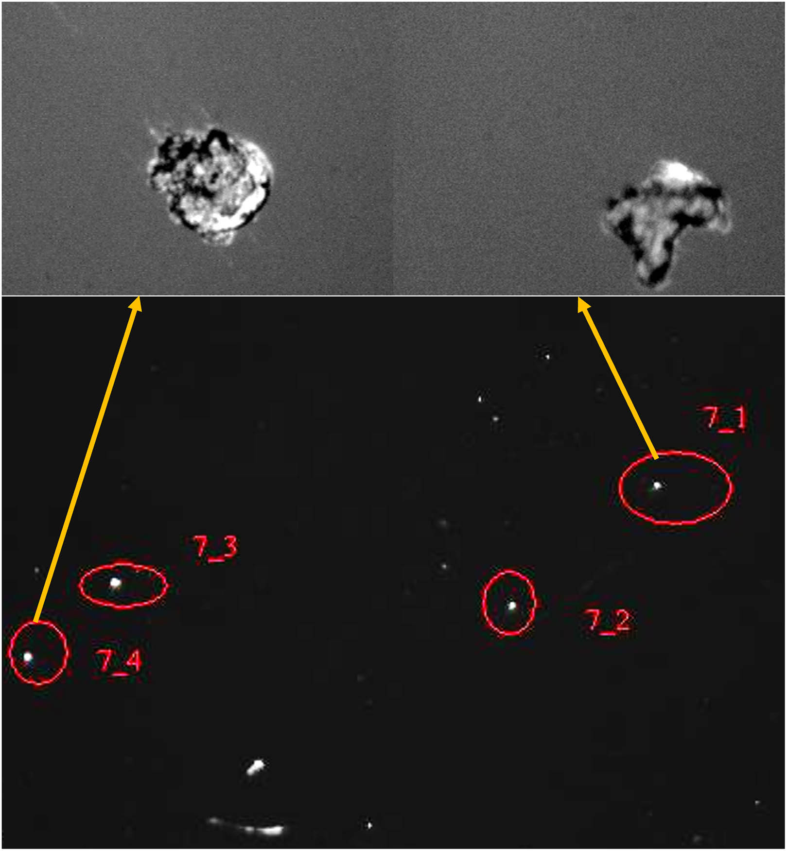
The size of LIDs is usually very small in the initial stage (<100μm). The in situ inspection method has shown great potential value by tracking the occurrence and growth of LIDs, and then shielding the local area of LIDs from upstream to reduce the local intensity and delay the growth of LIDs. This can greatly reduce the “catastrophic” damage caused by strong laser energy absorption due to LIDs and keep the output capability of the high-power laser. We have developed an in situ final optical element damage inspection (FODI) system^[1], which is an optical telescope designed to be inserted into the center of a target chamber after a laser shot. From this position, it can point to each beamline and acquire images (Fig. 1) of the optical elements. We have proved that the dark-field imaging is a high signal-to-noise detection method for the tiny LIDs under the condition of long working distances.

However, due to diffraction, optical aberration, and the slight defocus caused by poor focusing conditions of dark-field imaging, the imaging system suffers from blur degradation, which is expressed as Ic=Ig⊗κ,(1)where Ic is the image we actually captured, Ig is the ground-truth (GT) image, ⊗ denotes convolution, and κ represents the blur kernel of the optical system.

The degradation reduces the resolution of the image. Superresolution (SR) is required to improve the image resolution. But the sparse and tiny LIDs distributing in the dark background with little texture information cause more challenges to current image SR reconstruction methods.

Non-blind deconvolution is a suitable method^[2]. However, although the point spread function (PSF) is known, the PSF is usually band-limited (PSF itself also has accuracy and resolution limitations), so its frequency response shows zero or near-zero values at high frequencies. As a result, direct inversion of the PSF with the degraded image may cause large signal amplification at the high-frequency component, which manifests as ringing and amplified noise near the edges. Therefore, strong regularization is needed^[3,4].

Non-blind deconvolution using deep learning^[2] is superior to iterative deconvolution methods because it can tolerate greater model mismatch such as out-of-focus images, optical aberration, and PSF error^[5].

In 2020, a two-channel UNet^[6] model was proposed to solve the corrected images by separating the variables method and constructing multiple sub-optimization problems to solve them, which is relatively complex, although it works well. In 2021, the DWDN^[7] method explored Wiener deconvolution in deep feature space. It first performed Wiener deconvolution and then image reconstruction by an end-to-end network and obtained good results. However, the method performs poorly when the image contains many saturated regions or is heavily blurred. In 2021, a Uformer network was proposed that obtained good results on image reconstruction tasks but was computationally intensive. In 2022, a GAN-based deep convolutional neural network^[5] was proposed to perform deconvolution and SR on microscopy data encoded by known PSFs. The network uses simulated paired images based on known light propagation physics. It further uses unpaired real images for saliency checking; this thus reduces artifacts. But the GAN-based method is not easy to train and suffers from being crash-prone.

Inspired by NAFNet^[9], which obtained state-of-the-art results on the GoPro^[10] data set and MIMO-UNet^[11], which has an attractive feature fusion method, we propose a multichannel and multifrequency mixing deconvolution method that is suitable for the conditions of limited resolution, dark background, less texture, sparse and small lateral size, slight defocus, and PSF error of the damage detection image. This method can solve the problem of pixel alignment of high-low resolution sample pairs under such adverse conditions and achieve fine and reliable SR reconstruction results.

The proposed method consists of six steps, as shown in Fig. 2. In Step 1, we use a low-resolution imaging system to capture the images of a Bernoulli (0.5) random noise calibration pattern. We use the nonparametric subpixel local PSF estimation method^[12] to achieve high-precision PSF estimation of the low-resolution imaging system by calculating the tessellation angle of the calibration pattern using the line segment detection (LSD) algorithm, estimating the geometric variation of the camera, estimating and compensating illumination using the pattern matched with gray level, correcting the captured image to achieve an artifact-free PSF estimation using the sensor nonlinearity, as shown in Fig. 3. The relative error of the PSF estimation can be strictly limited to 2%–5%. Considering the inconsistency of the PSF at different positions in the image plane laterally, and in order to allow our model to learn the inverse process of the PSF at different lateral spatial positions in the image plane, we divide the imaging range into nine small regions and place the calibration pattern at random locations within each region, as shown in Fig. 4. We obtain nine laterally spatially varying PSFs. Considering that a slight defocus problem exists caused by poor focusing conditions of dark-field imaging, we change the distance between the optical element and the camera (with 10 mm steps in the range of 215–255 mm). We got 45 PSFs representing different distance and spatial positions.

In Step 2, we use a high-resolution imaging system to capture an image of the optical element, and the image is taken as the GT image.

In Step 3, we use these PSFs to convolve with the GT image to simulate the degradation effect image of the low-resolution imaging system. These calculated degraded images are naturally aligned with the GT image, and the magnification is consistent, forming a high-low resolution sample pair data set.

In Step 4, an end-to-end neural network (named MMFDNet) is proposed to carry out SR reconstruction of low-resolution images. We propose using a multifrequency information mixing block to cascade the whole network in the vertical direction, allowing flexible information delivery of features from top to bottom and from bottom to top. In order to enhance the feature information representation during the training phase, the network inputs the calculated low-resolution images, extracts multichannel and multifrequency information, and then gradually reconstructs the low-, intermediate-, and high-frequency information of the SR images.

In Step 5, the reconstructed results are supervised by the GT image using loss function and residuals backpropagation, so that the effects of defocus, diffraction, and noise degradation are removed from the results.

The structure of the deconvolution network (MMFDNet) proposed in this article is shown in Fig. 5; it is essentially an improved UNet^[8], where w represents the width of the network, H and W represent the height and width of the image, ⊙ represents concat, Ⓡ represents reshape, and ⊛ represents matrix multiplication. The network is divided into two parts: encoder and decoder. The encoder undergoes four downsamplings to extract features from high frequency to low frequency. The decoder undergoes four upsamplings to reconstruct images of different frequencies, from low to high.

The skip connections in existing improved UNet networks do not fully utilize different frequency information in the decoder image reconstruction process. In order to apply the information extracted by the encoder at different frequencies to the reconstruction process of each frequency of the decoder, this paper designs a multiscale channel feature fusion (MCFF) module, as shown in Fig. 5(d). We cascade the entire network in a vertical direction to achieve multiscale feature cross fusion, allowing for information flow from top to bottom and bottom to top. Multiple scale features can be fused at specified scales, enabling different scales to participate in calculations together. Compared to the original skip connection, it adds processing modules for fused features and has stronger representation capabilities. In addition, the MCFF module uses a resize operation to unify the scales to the corresponding dimensions, merge features together, and achieve the superposition of channel numbers, which can completely preserve all channel information and facilitate SR reconstruction.

In order to moderately alleviate the complexity increase caused by the above mixing, an NAF block was designed in the network, consisting of layer normalization (LayerNorm), a convolutional layer, a SimpleGate activation function layer, and a simplified channel attention (SCA) layer, as shown in Fig. 5(f). Layer normalization is carried out on different channels of each sample, ensuring stable and smooth training of the network.

The existing activation functions can be moderately simplified with gated linear units (GLUs)^[9] or Gaussian error linear units (GELUs)^[10]: GLU(x,f,g,σ)=f(x)⊙σ(g(x)),(2)GELU(x)=xΦ(x),(3)where x represents the input feature map, f and g are linear transformations, σ is a nonlinear activation function, such as Sigmoid, ⊙ represents the multiplication of elements, and Φ represents the cumulative distribution function representing the standard normal distribution. When f and g are set as unit functions, Φ takes σ GELU as a special case of GLU. GLU can replace nonlinear activation functions due to its generalization, and it itself contains nonlinearity and is not dependent on σ; even if the σ is removed, GLU still contains nonlinearity. Therefore, it is proposed to use SimpleGate instead of the nonlinear activation function, as shown in Fig. 5(c), to divide the feature map channel into two parts and multiply them, SimpleGate(X,Y)=X*Y,(4)where X and Y are feature images of the same size.

We introduce a moderately simplified channel attention to enable the network to adaptively adjust the weights of each channel in the feature map. Using global spatial feature information for feature compression, the two-dimensional information on each channel is transformed into a real number, and the weights of different channels are further calculated through the fully connected layer. Channel attention can be seen as a special case of GLU, CA(X)=X*Ψ(X),(5)SCA(X)=X*Wpool(X),(6)where CA(X) represents the original channel attention, and SCA(X) represents the simplified channel attention. Compared to the original channel attention, the simplified channel attention has more advantages in terms of computational complexity and parameter quantity, as shown in Fig. 5(d).

To validate the effectiveness of the proposed method, we need to obtain a data set consisting of high-low resolution sample data pairs. Therefore, we performed the experiment shown in Fig. 5, where we used edge illumination to illuminate the LIDs on the optical element^[1].

We obtained third-party high-resolution images using a camera (MER-1810-21U3C, pixel resolution, 4912×3684pixels) and a lens with high optical resolution (LMM-3XMP with an optical back focal length of 20.4 mm and magnification of 0.3× to 1.0×). We placed the high-resolution camera on a three-axis translation platform, which allows the camera to move horizontally, vertically, and back and forth. We used an LOG focus evaluation method to find the optimal focal position and obtain high-resolution images consistent with the lateral position of the damage point.

To measure the PSFs of the low-resolution imaging system, we used the nonparametric subpixel local PSF estimation method^[12], which requires the acquisition of Bernoulli (0.5) random noise calibration pattern images. As shown in Fig. 5, we used the same camera with a low optical resolution lens (M1214-MP2 F# 1.4, focal length 12 mm), and we placed the Bernoulli calibration plate on the front surface of the actual optical element to measure the PSF of the imaging system.

To construct high-low resolution sample pairs, we cropped the acquired high-resolution images and obtained 550 high-resolution sample images with sizes of 64 × 64 pixels. It was convolved with the 45 measured PSFs separately according to Eq. (1), and a data set of 550×45=24,750 high-low resolution image pairs data set was obtained.

For obtaining low-resolution images for testing, we used LOG focus evaluation to find the best focus position near the 215 mm distance. We used the same low-resolution lens (whose PSF has been measured) and camera to acquire images at a lateral position aligned with the damage point.

Figure 6 shows one of a set of measured PSF images. We trained both NAFNet and MMFDNet networks separately using the Loss1 function on the obtained damage data set and compared the reconstruction results. The experiments show that our proposed MMFDNet can reconstruct most of the detailed information and obtain high-resolution images with sharper edge information. It has a PSNR of 38.2017 dB (average value), which is 0.962 dB higher than that of NAFNet, and an SSIM of 0.983 (average value), which is 0.2% better than that of NAFNet. As shown in Fig. 7 and the data in Table 1, the output of MMFDNet obtained higher evaluation scores on the validation set images generated by the convolution of high-resolution images.

As shown in Eq. (2), the Loss1 function is a pixel-by-pixel comparison method. It has same weight for every pixel. This means that it devotes the same amount of attention to each pixel in the image, Loss1=1m∑i=1m|yi−f(xi)|.(7)

However, we are more concerned with the damaged region rather than the black background parts. Therefore, we design a new loss function with weight for the dark-field image. It assigns a greater weight to the damaged region than the background region. As in Eq. (3), we use the threshold segmentation method to separate the damaged region from the background. An additional term of the average absolute value error of the damaged region with weight is added to enhance the weight on the damaged region, as follows: $$\begin{gathered} Lossregion=Loss1+ω·1b∑iϵB|yi−f(xi)| \\ =1m∑i=1m|yi−f(xi)|+ω·1b∑iϵB|yi−f(xi)|, \end{gathered}$$(8)where m is the total number of image pixels, b denotes the number of pixels in the damaged region, ω is the size of the additional weight added to the damaged region, and B represents the set of pixels in the damaged region.

To determine the damaged region B, an adaptive mean thresholding segmentation method^[1] was used, since the method can achieve good segmentation results on our samples (Fig. 8).

Considering the damaged area is small, if ω is too large it may cause excessive attention problems and degrade performance. Therefore, in order to get appropriate ω, we used a random search method for the weight ω in the interval of 0–1.0. Figure 9 plots the results of the parameter search on our network. Our loss function performs better than Loss1 value in PSNR and SSIM values when the ω takes some specific values. Our network works best when ω=0.1297.

Table 2 shows the results of the comparison. It shows that our proposed MMFDNet and Lossregion achieve better performance on the data set: the PSNR is improved 1.333 dB, and the SSIM is improved 0.3% (average value).

Figure 10 shows the results for the images acquired with the low-resolution lens, and the results show that our method achieves better results.

In summary, we propose a multichannel and multifrequency mixing deconvolution method that is suitable for the conditions of limited resolution, dark background, less texture, sparse and small lateral size, slight defocus and PSF error while maintaining better PSNR and SSIM values. The experimental results prove the effectiveness of the method.

References

[6] Y. Nan, H. Ji. Deep learning for handling kernel/model uncertainty in image deconvolution. Proceedings of the IEEE/CVF Conference on Computer Vision and Pattern Recognition(2020).
[8] Z. Wang, X. Cun, J. Bao et al. Uformer: a general U-shaped transformer for image restoration. Proceedings of the IEEE/CVF Conference on Computer Vision and Pattern Recognition(2022).
[9] L. Chen, X. Chu, X. Zhang et al. Simple baselines for image restoration. Computer Vision–ECCV 2022(2022).
[10] S. Nah, T. H. Kim, K. M. Lee. Deep multi-scale convolutional neural network for dynamic scene deblurring. Proceedings of the IEEE Conference on Computer Vision and Pattern Recognition, 257(2017).
[11] S.-J. Cho, S. W. Ji, J. P. Hong et al. Rethinking coarse-to-fine approach in single image deblurring. Proceedings of the IEEE/CVF International Conference on Computer Vision(2021).
Set citation alerts for the article
Please enter your email address
© Copyright 2018-2021 | Chinese Laser Press. All Rights Reserved 沪ICP备15018463号-20