As is well known, owing to environmental changes or mechanical shocks, the state of polarization (SOP) of light emerging from telecommunication optical fiber links exhibits random temporal fluctuations, with corresponding SOP rotation speeds on the Poincaré sphere of up to 500krad/s [1]. Therefore there is a need for controlling or tracking the SOP of telecom signals whenever a polarization-dependent receiver is used. For example, in coherent systems, it is necessary to ensure the continuous matching among the SOPs of the received signal and that of the local oscillator. Currently, electro-optical SOP tracking is obtained via lithium–niobate waveguides driven by electronic feedback loops. Such polarization controllers operate in endless manner, namely without any resets that would possibly lead to data traffic interruptions or output intensity fluctuations as a result of sudden and large input signal SOP changes [2–5]. The technological development of these devices has improved their polarization tracking speeds from 0.1rad/s in early coherent systems [2] up to 59krad/s for use in 100Gbit/s transmission systems [5]. Moreover, in the current generation of long-haul transmission systems operating at channel rates of 100Gbit/s, pure electronic polarization tracking at rates in excess of 100krad/s can be performed thanks to the development of dedicated digital signal processing circuits [6,7].

Nevertheless, fully all-optical means to regenerate the signal SOP in fiber optics links will be required for the development of the next generation of transparent optical communication networks. As a matter of fact, in future transparent all-optical networks, several key functionalities such as optical add–drop multiplexing and optical cross connects will be implemented using silicon photonics integrated circuits (PICs). Since the operation of integrated optical waveguides requires a well-defined (e.g., TE) signal SOP, relatively complex and costly polarization diversity fiber-PIC coupling schemes, e.g., involving two-dimensional (2D) grating couplers, must be employed [8,9].

As we shall discuss in this paper, there is an alternative route for all-optical control of the signal SOP, which is based on the degenerate four-wave mixing (FWM) process in optical fibers [10–12]. Indeed, recent experiments have demonstrated two different methods for obtaining all-fiber, error-free regeneration of the SOP of 10 and 40Gbit/s on–off-keying (OOK) signals in standard telecom fibers. The first method involves the injection of a counter propagating continuous-wave (CW) pump [13–15] with a well-defined SOP. The second method simply exploits the nonlinear interaction of the signal with its back reflected replica obtained by connecting the fiber to a linear feedback mirror with adjustable reflectivity [16].

The operating principle of all-optical SOP tracking and regeneration in fibers is the so-called losslessness of the conservative polarization attraction effect. In the presence of a counterpropagating beam and for sufficiently intense wave powers and/or long fiber spans, all input signal SOPs are attracted toward a well-defined SOP at the fiber output. The attracting SOP thus acts as a sort of “polarization funnel,” as first described by Pitois and Haelterman in 2001 [17]. The resulting strength of signal repolarization is largely independent of its input SOP; quite remarkably, the operation of the nonlinear lossless polarizer is not accompanied by any loss of signal power, in marked contrast with the case of linear polarizers. On the other hand, in contrast with dissipative nonlinear polarizers based on Raman or Brillouin gain [18–23], in a lossless polarizer the input SOP fluctuations are not converted into output intensity fluctuations.

The first proof-of-principle demonstrations of the polarization attraction effect were obtained using counterpropagating nanosecond pump pulses and a short span of linearly isotropic highly nonlinear fiber [24–26]. A key breakthrough advance for the practical usage of nonlinear lossless polarizers in telecom applications consisted in the demonstration of signal repolarization induced by a sub-watt CW pump in a few-kilometer-long span of telecom nonzero-dispersion-shifted fiber (NZDSF) [13–15]. The relevance of this result, which was largely unexpected, stems from the fact that it demonstrates the robustness of the nonlinear polarization attraction even in the presence of a locally much stronger linear anisotropy or birefringence, which varies randomly along the fiber.

In fact, as theoretically demonstrated by Kozlov et al. [27], the rapidly varying random linear birefringence can be effectively averaged out from the propagation equations describing the nonlinear cross-polarization interaction between the signal and the counterpropagating pump. The availability of a simple deterministic model for describing nonlinear lossless polarizers based on randomly birefringent fibers provides a crucial tool for assessing their performance.

From the practical viewpoint, an important parameter is the maximum operating speed of a nonlinear lossless polarizer. In fact, theory and experiments agree well in evaluating the signal propagation delay through the fiber span as a typical estimate of the response time of the nonlinear polarizer [28]. As a result, polarization tracking speeds of 200krad/s could be reached when using a 6-km-long NZDSF [29]. Nonlinear SOP regenerators may have their operating power levels and required fiber length greatly reduced (hence tracking speed correspondingly increased) by using highly nonlinear and birefringent or spun optical fibers [30].

Since polarization attraction is based on the virtually instantaneous Kerr response mechanism of silica fibers, ultrafast signal polarization control may be achieved by exploiting the nonlinear cross-polarization interaction with a copropagating CW pump at a different carrier frequency [31]. Quite interestingly, a recent theoretical study by Kozlov et al. [32] has demonstrated that, in the copropagating configuration, the efficiency of signal repolarization grows larger as the temporal walk-off between the signal pulses and the CW pump is increased.

In Section 2, we will present a detailed experimental comparative study of the performance of the two different implementations of a nonlinear lossless polarizer for the regeneration of the SOP of 40Gbit/s OOK return-to-zero (RZ) signals. The initial setup involves an independent CW counterpropagating pump; as we will see, the degree-of-polarization (DOP) of the initially polarization scrambled signal grows monotonically larger until it reaches nearly unity at the fiber output as the pump power is increased above 800 mW. In the second setup, we replaced the pump beam by an adjustable feedback loop with variable reflectivity; here the output signal DOP exhibits a sudden transition to unitary values when the backreflected signal power gets larger than 500 mW, or the feedback loop reflectivity R>1. By means of bit-error-rate (BER) measurements, we will characterize and compare the power penalty of the two types of polarization regenerators. Quite interestingly, the setup with the reflective feedback loop shows 1 dB receiver sensitivity improvement with respect to the back-to-back (BB) configuration, indicating that polarization regeneration is accompanied by significant useful pulse shaping.

In Section 3, we briefly review a theoretical description of the phenomenon of polarization attraction. In substance, the theory makes use of recently developed mathematical techniques for the geometric study of Hamiltonian singularities [33]. This mathematical approach has been successfully applied to describe different configurations of polarization attraction in isotropic, high-birefringence, or spun fibers [34–38]. In substance, the theory reveals the essential role that the peculiar topological properties of singular tori play in the process of polarization attraction. This role may be interpreted intuitively by analogy with the role that plays a separatrix in purely one-dimensional (1D) systems. We remark that the existence of these singular structures had been essentially ignored in the physics literature until their recent introduction in the domain of atomic and molecular systems [39]. In this article we illustrate the theory in the particular example of polarization attraction in random birefringent fibers. We refer the interested reader to [36] for a recent article that reviews a pedagogical introduction to these mathematical tools as well as their applications to polarization attraction in different configurations.

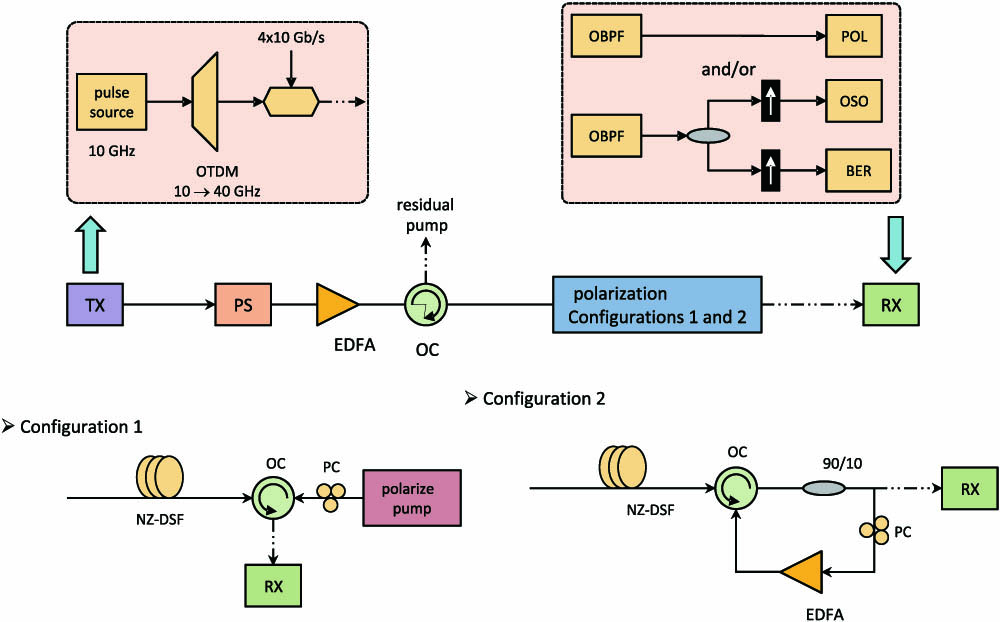
Throughout this paper, we consider an initial signal carrying RZ optical data with fast variations of its polarization state. The initial signal is injected into a low-polarization mode dispersion (PMD), normally dispersive optical fiber. A second wave also propagates in the same fiber in the opposite direction. Throughout the paper we are going to consider two different configurations, depending on the way the counterpropagating pump is generated. The first configuration corresponds to the case in which the pump wave results from an external source, whereas the second configuration, called the omnipolarizer, corresponds to the case in which the pump wave is replaced by a replica of the signal wave obtained by means of an active system of reflection.

The regeneration of the SOP of a 40Gbit/s RZ signal was experimentally achieved thanks to the experimental setup shown in Fig. 1. The 40Gbit/s RZ signal was generated by means of a 10 GHz mode-locked fiber laser delivering 2.5 ps pulses at 1564 nm. A programmable liquid-crystal-based optical filter allows us to temporally spread the initial pulses so as to obtain 7.5 ps Gaussian pulses through a spectral slicing operation. The resulting pulse train was intensity modulated thanks to a LiNbO3 modulator through a 231−1 pseudo-random bit sequence. A two-stage bit-rate multiplier was used to generate the initial 40Gbit/s RZ bit stream. Large and fast fluctuations of the signal polarization were induced via a polarization scrambler (PS) working at a rate of 650 Hz. Before injection into the optical fiber, the 40Gbit/s signal was finally amplified by means of an erbium-doped fiber amplifier (EDFA) at the suitable average power of 27 dBm. The optical fiber involved in the FWM-based polarization attraction process is a 6.2-km-long NZDSF with the following parameters: chromatic dispersion D=−1.5ps/nm/km at 1550 nm, nonlinear Kerr parameter γ=1.7W−1·km−1, and PMD coefficient Dp=0.05ps/km1/2. Two optical circulators were inserted at both fiber ends, so as to inject and collect both waves.

As mentioned above, the counterpropagating wave, which acts as the polarization attractor wave, results either from an external source or from a reflection of the signal. The external pump wave (i.e., the configuration 1 depicted in Fig. 1) consists of a 1 W continuous incoherent wave having a fixed arbitrary SOP, a spectral linewidth of 100 GHz, and a central wavelength of 1545 nm. On the other hand, the output reflective element (i.e., involved in configuration 2 depicted in Fig. 1) is composed of a fiber coupler (90/10), a polarization controller, and an EDFA. Let us define the reflection coefficient R as the ratio between powers of the reflected signal and the initial input wave. Thanks to the active control loop, R can be lower than, equal to, or superior to unity. At the receiver, a polarizer was inserted in order to translate the polarization fluctuations into intensity fluctuations. Behind the polarizer, the 40Gbit/s eye diagram was monitored by means of an optical sampling osvfcilloscope (OSO), while the BER was measured thanks to a fast photodiode (70 GHz bandwidth) followed by electrical demultiplexing at 10Gbit/s. Note that the BER measurements were averaged on the four resulting demultiplexed 10Gbit/s channels. The 40Gbit/s signal SOP was recorded onto the Poincaré sphere using a commercially available polarimeter (POL).

The transfer function of the polarization regenerator was experimentally measured by evaluating the DOP as a function of pump power. DOP is classically defined as DOP=〈S1〉2+〈S2〉2+〈S3〉2/S0, where Si are the Stokes parameters of the signal wave and 〈〉 denotes an averaging over 256 runs of input polarizations. As can be seen in Fig. 2, the DOP of the signal wave, which initially has a low level due to its initial scrambling, strongly increases when the counterpropagating pump power is injected into the fiber so as to saturate and reach asymptotically a constant value close to unity for a pump power above 800 mW. Based on these results, a pump power of 1 W was chosen to ensure a maximum efficiency of the polarization attraction process.

The performances of the polarization regenerator were quantified in realtime by means of the SOP monitoring and eye-diagram visualization as illustrated in Fig. 3. At the regenerator output and in the absence of a counterpropagating pump wave, because of the initial polarization scrambling process, the signal SOP is uniformly spread onto the whole Poincaré sphere [Fig. 3(a1)], leading to a complete closure of the eye diagram [Fig. 3(b1)]. Indeed all the polarization fluctuations generated by the PS are transformed into intensity fluctuations through the polarizer, thus inducing a complete eye closure and loss of data. On the other hand, in the presence of the polarized pump wave [Figs. 3(b)], the polarization attraction process leads to the convergence of all polarization states toward a small area on the Poincaré sphere [Fig. 3(b1)], indicating an efficient stabilization of the 40Gbit/s signal SOP. The output eye diagram depicted in Fig. 3(b2) becomes now completely open behind the polarizer, confirming the high efficiency of the regeneration of the polarization process.

Finally, Fig. 3(c) shows the BER measurements of the 40Gbit/s signal as a function of the incoming power on the receiver. For reasons of clarity, Fig. 3(c) only shows the average value of the BERs obtained for the four demultiplexed 10Gbit/s channels. The reference is illustrated by the BB configuration (i.e., at the fiber input). As shown by the eye diagram reported in Fig 3(a), at the output of the regenerator, when the polarization of the signal is scrambled, the BER is limited by an error floor at 10−2. But remarkably, in the presence of the counterpropagating pump wave (dark circles), the quality of the transmission is greatly improved, and negligible power penalty at the error-free level (i.e., for BER=10−9) with respect to the BB case was obtained at the receiver.

In the previously discussed configuration involving a separate pump beam, the signal SOP obtained at the regenerator output depends on the initial SOP of the pump. As we shall see next, quite remarkably in the second configuration with the adjustable reflective device (omnipolarizer), the regenerated signal is circularly polarized no matter the SOP of the backreflected wave, although its ellipticity (right or left) may be adjusted by means of a linear polarization controller. Figure 4(a) shows the evolution of the signal SOP at the omnipolarizer output for different values of the reflection coefficient R. As can be seen, for R=0.32, the polarization attraction process starts to develop, and the points localized in the north (south) hemisphere, corresponding to right (left) SOPs, start to converge on the north (south) pole of the Poincaré sphere. When R is equal to 0.68, this convergence is more pronounced and the output SOPs are confined around both poles of the sphere—that is, close to the right- or left-handed circular polarizations. In other words, depending on its initial ellipticity, all of the 40Gbit/s signal energy is digitally routed to either the right- or left-circular SOP without any pulse splitting. When R=0.78, the attraction zone, which was previously localized around the south pole, explodes and all of the corresponding output SOP points on the Poincaré sphere are now attracted toward the north pole. When R=1.14, all the SOPs of the output signal wave converge around the north pole, so that the signal polarization remains close to a right-handed circular SOP. In other words, the signal light has self-organized its own SOP. Let us point out that the signal ellipticity at the regenerator output for R greater than unity is dependent on the polarization controller inserted into the reflective loop (see Fig. 1). Indeed, according to the transfer function of the polarization controller, all of the signal SOPs converge either to the north pole or to the south pole of the Poincaré sphere. Consequently, by tuning the polarization controller, no matter the initial SOP, it is possible to ensure that the output signal polarization remains trapped close to either a right-handed or a left-handed circular polarization state. It can be noted that the selection of either the right- or left-circular SOP is determined by the angle of polarization rotation in the reflection process. Such angle is at the origin of the symmetry breaking between the two circular SOPs, and it can be adjusted experimentally thanks to the polarization controller. More precisely, if one only considers a polarization rotation around the vertical axis of the Poincaré sphere, then a positive (negative) rotation angle favors the left- (right-) circular SOP (see [16] for more details).

We measured the DOP of the output signal for a large number of values of R, and the results are summarized in Fig. 4(b) as a function of the average power of the reflected signal (or similarly as a function of R). It is interesting to point out that, in contrast with the configuration based on an external pump where the DOP increases monotonously until saturation, in this case the evolution of the output DOP clearly exhibits a minimum. To comment on Fig. 4(b) in more detail, let us first remember that the omnipolarizer operates in two distinct regimes depending on the reflection coefficient R, the polarization beam splitter (PBS) regime, and the polarization regime [16]. For a depolarized input signal (DOP=0), numerical simulations (not shown here) indicate that the PBS regime operates for 0.67<R<0.83, while the polarization regime operates for R>1. However, the situation in Fig. 4 is more complex because the injected signal is not depolarized, but it is partially polarized; i.e., for a weak reflected power (Pr<100mW) in the linear regime, its DOP∼0.19. As the reflected power increases, namely for 310mW<Pr<345mW, the device operates in the PBS regime, whose efficiency reaches its optimal value for Pr=340mW (corresponding to R=0.68). In this PBS regime there exists a strong attraction toward both the north and the south poles, which merely explains the decrease of the DOP (down to ∼0.02). We remark here that the value of R=0.68 is close to the lower limit of the expected interval of PBS operation (0.67<R<0.83). Numerical simulations indicate that this can be ascribed to the fact that the injected wave is partially polarized, which permits the system to enter the PBS regime with a reflected power that is slightly smaller than the value that would be expected if the input signal was fully depolarized. Finally, for a reflected power Pr>500mW, the system enters the polarization regime, characterized by a polarization attraction toward the north pole, which leads to an increase of the DOP close to the unit value. We note that the system enters the polarization regime for a reflection coefficient close to the expected value (i.e., for R∼1). This remarkable evolution of the DOP can be clearly understood by means of the Poincaré spheres shown in Fig. 4(a). For example, the minimum value of the signal DOP is obtained when points remain trapped close to either the north pole or the south pole.

Following the example of the previously described study involving an independent pump beam, we have also visualized the eye diagrams at the omnipolarizer output without (R=0) and with (R=1.2) the reflected signal wave, as shown in Fig. 5(a). We can clearly notice that the reflection of the signal leads to a complete opening of the eye, thus demonstrating the efficiency of the omnipolarizer to regenerate the polarization of a 40Gbit/s signal. More importantly, the corresponding BER measurements [see Fig. 5(b)] show that, despite the initial polarization scrambling process, the omnipolarizer enables clean error-free data recovery behind a polarizer. Indeed, Fig. 5(b) even shows a 1 dB receiver sensitivity improvement with respect to the BB configuration, thus indicating that polarization regeneration is accompanied by significant and useful pulse shaping as well.

The description of the previously discussed phenomenon of polarization attraction can be made on the basis of the analysis of the spatiotemporal dynamics of two counterpropagating beams in a randomly birefringent telecom fiber. The evolution of the polarization of the beams is governed by the following equations derived in [28]: $$\begin{gathered} ∂S⃗∂t+∂S⃗∂z=S⃗×(IJ⃗) \\ ∂J⃗∂t−∂J⃗∂z=J⃗×(IS⃗). \end{gathered}$$(1)

These equations are written in a rotating reference frame in order to discard the linear birefringence terms. In Eq. (1), the polarization states of the forward and backward beams on the Poincaré sphere are described by the Stokes vectors S⃗=(Sx,Sy,Sz) and J⃗=(Jx,Jy,Jz), respectively. The sign “×” denotes the vector product, and I is the diagonal matrix defined by diag(−1,−1,1). No fiber loss has been taken into account in the model. The numerical simulations of Eq. (1) reveal that such terms have a minor effect on the polarization attraction process. In this case, the beam powers S0=Sx2+Sy2+Sz2 and J0=Jx2+Jy2+Jz2 are conserved quantities. To simplify the notations, the problem has been normalized with respect to the characteristic nonlinear time τ0=1/(γS0) and length Λ0=vτ0, of the system, where v denotes the group velocity of the waves into the fiber and γ is the nonlinear Kerr coefficient. In spite of its apparent simplicity, the model given in Eq. (1) captures the essential properties of the polarization attraction in a telecommunication optical fiber. Note that models of the form (1) are quite general, in the sense that the same equations, though with a different form of the matrix I, describe light propagation in isotropic fibers, high-birefringence fibers, or spun fibers [36].

The physical mechanism underlying the observed polarization attraction phenomenon can be described in terms of mathematical techniques developed for the study of Hamiltonian singularities (see [34,36,38] for recent papers on the subject). This geometric approach proved efficient in describing polarization attraction in different circumstances. Here we briefly summarize the method for the example of the random birefringence fibers. The first step of the study consists in analyzing the stationary states of the system, which are ruled by the following ordinary differential equations: ∂Sx∂z=SyJz+SzJy∂Sy∂z=−SxJz−SzJx∂Sz∂z=−SxJy+SyJxand∂Jx∂z=−SyJz−SzJy∂Jy∂z=SxJz+SzJx∂Jz∂z=−SxJy+SyJx.(2)

Equations (2) have a Hamiltonian structure [33] defined by the Hamiltonian function H, which is a constant of the motion: H=SxJx+SyJy−SzJz.

Due to the symmetry of the system, there are three other constants of the motion Kx=Sx+Jx, Ky=Sy+Jy, and Kz=Sz−Jz. It can be shown that the corresponding stationary system is Liouville integrable [33], which means that the orbits are contained on invariant tori in the associated phase space representation. Such torus can be either regular or singular depending on the values of the different constants of the motion. In this case, the regular tori can be viewed as 2D structures that are topologically equivalent to a doughnut. On the other hand, singular sets are peculiar geometrical objects that cannot be deformed continuously into a regular torus. We refer the reader to [36] for an introductory approach to these mathematical concepts. Singular sets can be of different types, e.g., points of equilibrium, periodic orbits, or 2D extensions of the concept of separatrix, which is a well-known property of basic 1D physical systems. In the present model, the singular set is composed of families of points of equilibrium. The characteristic properties of singular sets can be determined from a general mathematical method known as “singular reduction theory” (see [33] for details). The basic idea of the theory is the reduction of the dimension of the phase space representation by making use of a constant of the motion. Applying this theory to all possible values of H and the three constants Ki, one can construct the so-called energy momentum representation. This diagram is represented in Fig. 6 for the particular case where S0=J0=1. We choose to plot this diagram as a function of Kz, but an equivalent figure would be obtained with the two other constants. Without entering into details, it can be shown that any point of the diagram can be associated to a regular torus, except for the singular point, which is located at H=−1 and Kz=0 (note that the boundary of the diagram also refers to singularities, which correspond to either circles or points [36]). For the present model, the singular set corresponding to the singular point can be represented as a sphere, an object that is istopologically singular in the sense that it cannot be transformed in to a regular torus by means of continuous deformations. The key point to underline here is that the orbits associated with the singular set will be shown to play the role of an attractor for the spatiotemporal dynamics [34], an important feature that will be illustrated below with numerical simulations of the complete Eqs. (1). Accordingly, the properties of the singular point in the energy momentum representation (H,K) in turn determine the properties of the phenomenon of polarization attraction.

Let us first illustrate this aspect with the two-source configuration of polarization attraction (termed configuration 1 in Section 2), in which a pump beam is injected at the fiber output with the SOP J⃗(L)=(Jx(L),Jy(L),Jz(L)). Since the singular set of interest is defined by H=−1, Kx=0, Ky=0, Kz=0, one deduces that the signal SOP at z=L is S⃗(L)=(−Jx(L),−Jy(L),Jz(L)). The same reasoning can be used for the omnipolarizer configuration (configuration 2) of polarization attraction. In this case, the mirror boundary conditions at z=L force the system to be in two unique SOPs, which correspond to the two states of circular polarization: S⃗(L)=(0,0,±1). Note that we pass from one point of attraction in the standard configuration to two points when the mirror conditions are considered.

These theoretical predictions are remarkably well confirmed by numerical simulations. In many cases of interest, one observes that the counterpropagating waves relax, after a complex transient, toward a stationary state. We report in Fig. 7 the polarization states at the fiber output (z=L) once the transients have died out, for both polarization attraction configurations, i.e., the traditional two-source configuration (1) and the omnipolarizer configuration (2). In configuration 1, we observe that the signal wave is attracted (up to a sign change) to the injected pump SOP at z=L, S⃗(L)=(−Jx(L),−Jy(L),Jz(L)). Conversely, in the omnipolarizer configuration 2, attraction always occurs on the poles of the Poincaré sphere, i.e., the circular polarization states. Note that the efficiency of the attraction process increases as the fiber length increases, a property that can be explained from the above theory (see [34]). It is also interesting to note in Fig. 7 that polarization attraction is more efficient in the omnipolarizer configuration as compared to the traditional two-source configuration.

We finally briefly discuss the response time of polarization attraction through analysis of the trajectory of the signal SOP on the surface of the Poincaré sphere. As commented above, the space-time dynamics can be characterized by a complex transient whose structure depends on the boundary condition imposed at z=0 of the omnipolarizer (or at both ends of the fiber in the two-source configuration). When the optical beam enters the optical fiber at z=0 (i.e., when the laser is “switched on”), its intensity varies progressively from 0 to a stationary value (and stationary SOP). Let us call τtr the time required to reach such a stationary state. If this time is much larger than the time required for the beam to propagate throughout the system, i.e., τtr≫τL=2L/vg, then the waves adiabatically follow an instantaneous stationary state: the signal SOP evolves essentially in a monotonic way toward its attraction polarization state, as illustrated in Fig. 6(d). Conversely, when τtr∼τL, the system does not have sufficient time to adiabatically follow the rapid variations of the injected beam (at z=0), and thus the signal SOP exhibits a complex erratic transient before reaching its final attraction polarization state [see Fig. 6(c)]. The impact of the boundary conditions on the response time of the repolarization process is also clearly visible in the energy momentum representation, as illustrated in Figs. 6(a) and 6(b); as opposed to the erratic behavior, in the adiabatic limit the system relaxes toward the singular torus in a monotonic way (see [35] for a theoretical approach of this adiabatic repolarization process).

In conclusion, we have reported the experimental demonstration of all-optical polarization regeneration of 40Gbit/s RZ signals at telecommunication wavelengths. Our technique involves a FWM-based attraction process between an incident arbitrarily polarized signal with a counterpropagating control pump taking place in a 6.2-km-long normally dispersive NZ-DSF characterized by low PMD. We have considered two configurations: the one in which the pump is delivered by an external source, termed the two-source configuration, and the one obtained by reflection of the signal at the fiber output, called the omnipolarizer. By using a small amplification of the reflected signal, the omnipolarizer leads to similar results to those obtained with an external pump. In particular, in both configurations the input signal with a random polarization emerges from the regenerator with a stabilized SOP and without intensity fluctuations. However, the omnipolarizer presents the advantage of a simplification of the device and is more efficient when compared with the traditional two-source configuration. Indeed a DOP close to 1 is obtained, on the one hand with an external pump power larger than 800 mW, and on the other hand with a reflected signal power larger than 500 mW. Based on our experimental observations, we think that these two polarization regenerator configurations could find many applications in all-optical signal processing for future transparent optical networks. In particular our device can be of interest for legacy and cheap fiber optic transmission systems with direct detection and that do not use polarization division multiplexing.

In perspective, we could envisage to explore the capacity of our polarization regenerators to operate with optical data streams that are multiplexed in wavelength. Similarly, it would be interesting to study the efficiency of the polarization regenerators for other modulation formats, such as polarization dense multiplexing or phase shift keying. Finally, another interesting perspective could be dedicated to the use of highly nonlinear fibers (such as chalgonenide or fluoride fibers) in order to reduce the fiber lengths and the required optical powers.

We finally note that the theoretical approach considered here is general and can be applied to the study of polarization attraction in different configurations. For instance, high-birefringence spun fibers exhibit a phenomenon of polarization attraction of a different nature than that discussed here [38]. In spun fibers, attraction does not occur toward a particular polarization state, but instead toward a specific line of polarization states on the surface of the Poincaré sphere. This shows that the properties of the phenomenon of polarization attraction strongly depend on the properties of the particular optical fiber under consideration. Besides the characterization of the phenomenon of polarization attraction, the theory exposed here can also be extended to study the stability properties of soliton solutions in a medium of finite extension [40,41]. Work is in progress to extend this preliminary work to more general soliton systems, such as gap solitons and three-wave interaction solitons.

Acknowledgment. We acknowledge the insightful contribution to the theoretical description of polarization attraction of Victor V. Kozlov, who unfortunately could not see the completion of this work because of his decease. We will remain grateful to Victor for the many discussions we shared and his enthusiasm. All the experiments were performed on the PICASSO platform in ICB. We acknowledge financial support from the European Research Council under the Grant Agreement 306633 PETAL ERC project, the CNRS, the Labex ACTION program (contract ANR-11-LABX-01-01), and the Conseil Régional de Bourgogne under the PHOTCOM program.

References

[1] M. Reimer, D. Dumas, G. Soliman, D. Yevick, M. O’Sullivan. Polarization evolution in dispersion compensation modules, OWD4(2009).
[29] V. V. Kozlov, J. Fatome, P. Morin, S. Pitois, S. Wabnitz. Nonlinear optical fiber polarization tracking at 200 krad/s. 37th European Conference on Optical Communication (ECOC), 2011(2011).
J. Fatome, D. Sugny, S. Pitois, P. Morin, M. Guasoni, A. Picozzi, H. R. Jauslin, C. Finot, G. Millot, S. Wabnitz, "All-optical regeneration of polarization of a 40 Gbit/s return-to-zero telecommunication signal [Invited]," Photonics Res. 1, 115 (2013)