
S. Gerlach, F. Balling, A. K. Schmidt, F. E. Brack, F. Kroll, J. Metzkes-Ng, M. Reimold, U. Schramm, M. Speicher, K. Zeil, K. Parodi, J. Schreiber. Three-dimensional acoustic monitoring of laser-accelerated protons in the focus of a pulsed-power solenoid lens[J]. High Power Laser Science and Engineering, 2023, 11(3): 03000e38
- High Power Laser Science and Engineering
- Vol. 11, Issue 3, 03000e38 (2023)
Abstract
1 Introduction
Over the past few decades, high-power laser systems have been the subject of increasing scientific interest for various applications, resulting in more than 50 systems worldwide with peak powers of more than 200 TW that have been in operation, are operational or are in the construction or planning phase[1]. One of their multidisciplinary applications is the acceleration of charged particles, such as protons or ions, generated by the laser being focused onto a target[2,3]. The acceleration in a plasma provides highly energetic protons with properties that are complementary to radiofrequency (RF) acceleration, in particular by ultra-high peak intensities[4,5]. Potential applications of laser-driven proton sources are in biomedical physics, nuclear physics and material research[2,3,6]. Dedicated beamlines for proton bunch manipulation have been developed to transport and focus a selected part of the ion spectrum emitted from the plasma to a small spot with a typical size of a few mm[7–9]. This technological advance has recently enabled tremendous progress in radiation-biological applications[9–11].
Online characterization of these focused ion bunches has remained a challenge[2,12]. One promising approach relies on measuring the acoustic wave excited by the ions stopping in water by ultrasonic transducers[13–16]. Recently, this ionoacoustic method was employed for reconstructing the proton bunch energy distribution from a single acoustic trace, dubbed I-BEAT (Ion-Bunch Energy Acoustic Tracing)[17]. The benefit of I-BEAT for laser-accelerated ions is the analogue delay of amplification and digitization due to the low speed of sound, which enables separation from prompt disturbances such as the electromagnetic pulse (EMP). In addition, the conversion of deposited energy density into pressure is linear over a large range of bunch intensities[18]. So far, I-BEAT has yielded the energy spectrum of an individual proton bunch by an iterative reconstruction algorithm that has also approximated the lateral bunch size by using only one ultrasonic transducer[17].
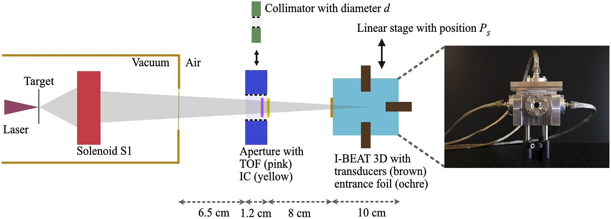
Figure 1.Schematic top view of the experimental setup (not to scale) with all components relevant for this study; in addition, a picture of the I-BEAT 3D detector is shown with the circular entrance window being visible in the centre of the detector. The laser (magenta) is focused onto a thin foil target (black) from which protons are accelerated (grey). One energy selective solenoid S1 focuses the protons to a spot in air. The protons pass either an aperture equipped with a time-of-flight spectrometer (TOF, pink) and an ionization chamber (IC, yellow), or a collimator with a variable diameter (green). Finally, the protons reach the I-BEAT 3D detector, which is positioned on a linear stage. I-BEAT 3D consists of a water reservoir (turquoise) surrounded by four ultrasonic transducers (brown, three are visible). The ions enter the water through a thin Kapton entrance foil (ochre).
Here we present an extension to I-BEAT 3D for analysing particle bunch properties in three dimensions. I-BEAT 3D is equipped with three additional transducers for improving the sensitivity to lateral bunch properties. Using simplified but fast filtered raw data analysis, this setup allows monitoring of the proton bunch mean energy and energy width, lateral position and lateral size as well as the bunch particle number directly from the four acoustic traces.
Sign up for High Power Laser Science and Engineering TOC. Get the latest issue of High Power Laser Science and Engineering delivered right to you!Sign up now
2 Materials and methods
2.1 Experimental setup
Figure 1 shows the experimental setup that is implemented at the ALBUS-2S ion irradiation beamline of the DRACO laser at Helmholtz-Zentrum Dresden-Rossendorf (HZDR Dresden)[8]. We operated solenoid S1 to select a small energy range around a design energy value between 13 and 31 MeV from the broad spectrum of laser-accelerated protons, which reached up to 54 MeV. Information on the bunch manipulation by the solenoids can be found in Ref. [8] along with an example of the transported spectrum. After exiting the vacuum chamber, the bunch travels through an air gap of 6.5 cm in length. Then, the proton bunch passes either an aperture equipped with a time-of-flight (TOF) spectrometer[11,19,20] and a parallel plate ionization chamber (IC, X-Ray Therapy Monitor Chamber 7862, PTW Freiburg) positioned behind the aperture connected to a dosemeter (UNIDOS, PTW Freiburg) to deduce the proton bunch particle number or a collimator of variable diameter between 1 and 5 mm. The bunch then enters the I-BEAT 3D detector, which is positioned 8 cm behind the aperture or the collimator, respectively. To allow accurate lateral shifts in the horizontal direction relative to the proton axis, the I-BEAT 3D detector is positioned on a motorized stage. I-BEAT 3D consists of an aluminium box with dimensions of 16 cm × 14 cm × 10 cm filled with water into which protons enter through a 50 μm thin Kapton entrance window. While the previous I-BEAT detector was equipped with only one ultrasonic transducer[17] positioned on the proton axis, the I-BEAT 3D design has four transducers chosen out of the Videoscan series, Olympus Deutschland GmbH. This series offers immersion transducers with various properties, particularly a variable frequency response represented by a central frequency. Furthermore, transducers with flat and spherical sensitive surfaces are available; the latter kind is further referred to as focused. One transducer is mounted in extension of the proton bunch axis (‘axial transducer’, 10 MHz central frequency, 2.54 cm focal length) and has a distance of 3 cm to the entrance window. The three lateral transducers are installed to the right (1 MHz, flat), left (1 MHz, flat) and top (3.5 MHz, 2.54 cm focal length) of the water volume. We chose transducers with lower central frequency for the lateral positions to account for the difference in the frequency spectrum of the acoustic wave at the lateral and axial transducer positions. This is due to the expected sharper gradient in energy deposition in the axial extent of the Bragg peak (BP). It is expected that the central frequency of the transducer influences the deduction of the lateral bunch width. To investigate this, transducers with two different central frequencies are picked for the right/left and top positions. While the top and the axial transducers are chosen to be focused for the optimal signal amplitude, the right and the left transducers are flat to support the scan of the lateral bunch position. For the study presented here, I-BEAT 3D is aligned such that the BP of 30 MeV protons is in the centre of the four transducers (besides when varying the lateral position of the detector relative to the bunch). The distance of each transducer to this design centre is 2.54 cm, which corresponds to the focal length of the axial and the top transducers. The signal of each transducer is 60 dB, amplified by a commercial low-noise amplifier (HVA-10M-60-B, Femto Messtechnik GmbH).
![]()
Figure 2.Exemplary ionoacoustic signal recorded with the (a) axial transducer and (b) the right lateral transducer. Curves represent the lowpass filtered data (red, cut-off frequencies:  MHz for the axial transducer and
  MHz for the right transducer) and the signal envelope (black). The read-out positions for the deduction of the bunch properties from the signal envelope are marked by dashed lines. For the axial transducer, the arrival time difference between the first and the third maxima corresponds to twice the proton bunch range
  , the pulse width
  is related to the width of the BP and the amplitude
  reveals the bunch particle number. For the lateral transducers, the position of the maximum
  is used to define the lateral bunch position and the pulse width
  relates to the lateral bunch diameter.
2.2 Data analysis
The duration of the proton bunch at the detector position is of the order of tens of ns, which is much smaller than the stress confinement time[21] that is typically a few μs. In this case, the initial pressure is the product of the energy density distribution deposited by the protons and the material-dependent Grüneisen parameter, which relates energy density to pressure. The propagating pulse amplitude is proportional to the spatial derivative of this initial pressure. Hence, if the deposited energy distribution exhibits only a single spike, such as the BP of focused protons, we expect a single-cycle pulse with a central wavelength and a pulse duration proportional to the size of the distribution in the respective direction of observation. As the phase and amplitude of the acoustic signal will be modified on detection, depending on the spatial and impulse response of the complete geometry and amplifier system[22], we restrict the analysis to the signal envelope calculated by taking the absolute value of the signals’ Hilbert transformation and deduce the amplitudes with their respective positions as well as their full width at half maximum (FWHM) values. Figure 2 shows an exemplary signal for both the axial and the right lateral transducers. The
2.2.1 Axial transducer signal
The axial signal in Figure 2(a) reveals three temporally separated pulses that are typical for proton bunches with narrow energy spread[14]: the first one corresponds to the acoustic wave emitted from the BP directly towards the axial transducer. Likewise, an acoustic pulse is emitted from the BP location in the opposite direction towards the entrance foil, where it is reflected and propagates towards the axial transducer, leading to the third peak. The arrival time difference between both pulse envelope maxima, marked by the vertical magenta lines, corresponds to twice the proton bunch range
The width of the pulse
The second pulse that appears in the centre of the signal trace is generated at the location of the entrance foil. We will show that this signal, in particular the amplitude of its envelope
2.2.2 Lateral transducer signal
Figure 2(b) shows a typical lateral signal recorded with the right transducer. At
3 Results
3.1 Axial bunch properties
Figure 3(a) shows the range
Figure 3(b) shows the I-BEAT 3D signal width
![]()
Figure 3.(a) Estimated mean energy and range as a function of the solenoid magnetic field for I-BEAT 3D (black) and TOF (blue). (b) I-BEAT 3D signal width as a function of the determined I-BEAT 3D mean energy. A fit of the I-BEAT 3D data dots according to Equation (
![]()
Figure 4.(a) I-BEAT 3D result of the bunch position in dependence of the stage position. The resolution limit is shown in red. (b) Measured lateral signal size in dependence of the collimator size along with a fit according to Equation ( is found to be
  mm for the right transducer and
  mm for the top transducer.
3.2 Lateral bunch properties
Figure 4 shows the lateral bunch position estimated from the I-BEAT 3D signal. The spatial resolution limit calculated by
Figure 4(b) shows the width of the ionoacoustic signal
![]()
Figure 5.The amplitude of the ionoacoustic signal envelope generated in the I-BEAT 3D entrance window is displayed in dependence of charge measured with the ionization chamber for various bunch particle numbers. In addition to the black data dots, the linear correlation curve is shown in green.
3.3 Bunch particle number
Figure 5 shows the amplitude of the window signal
4 Discussion and conclusion
Equipped with four transducers, the I-BEAT 3D detector provides acoustic traces in four spatial directions. As expected, the analysis of the envelope of the filtered raw signal amplitudes reveals the position and the width of the BP volume. The accuracy of this position is currently limited to the resolution limit of 0.04 mm in the axial dimension and 0.16 mm in the lateral dimension, depending on the maximal detectable frequency and the signal-to-noise ratio. In the axial direction, this analysis yields an absolute measure of the proton range[14,24] and hence kinetic energy before entering the water reservoir in real-time with an accuracy of 0.8 MeV. Analysis of the width of the signal envelope allows in addition fast monitoring of the width of the BP, which is a measure of the energy spread
Particularly interesting is the observed correlation between the ionoacoustic signal generated in the entrance window of the I-BEAT 3D detector and the IC signal, although the deviations are larger than the individual uncertainties. This hints at the differences due to the physics of the two approaches. While the IC measures the number of charges that is assumed to scale (eventually nonlinear) with the total particle number[6], the ionoacoustic signal depends on the spatial distribution of the bunch that traverses the entrance foil and on the detector geometry. That is, the signal is sensitive to proton bunch fluence, and not just particle number, which can be seen in Equation (1) in Ref. [17]. As an example for a 30 MeV proton bunch, when increasing the lateral signal width from 3 to 3.1 mm, the pressure amplitude is decreased by approximately 5%.
In conclusion, the presented fast and simple data analysis allows monitoring important proton bunch parameters of the focused and energy selected proton bunch in a compact, simple, fast and EMP-resistant online tool. Compared to the previously used simulated annealing approach[17] demonstrated for dose reconstruction in the axial dimension (i.e., the depth dose curve), the here presented fast data analysis has the advantage that the extraction of information becomes compatible with 1 Hz operation and potentially much higher repetition rates. Having in mind that a full reconstruction of the depth dose curve is possible, for many use cases fast feedback on the energy width of a focused proton bunch is sufficient. The I-BEAT 3D detection method is not only promising as a beam monitor for laser-ion accelerators, but could also be applied for preclinical and clinical research in the context of FLASH radiotherapy[6], as the high dose rates used in this new treatment modality challenge well-established bunch monitoring systems.
References
[1] C. N. Danson, C. Haefner, J. Bromage, T. Butcher, J.-C. F. Chanteloup, E. A. Chowdhury, A. Galvanauskas, L. A. Gizzi, J. Hein, D. I. Hillier, N. W. Hopps, Y. Kato, E. A. Khazanov, R. Kodama, G. Korn, R. Li, Y. Li, J. Limpert, J. Ma, C. H. Nam, D. Neely, D. Papadopoulos, R. R. Penman, L. Qian, J. J. Rocca, A. A. Shaykin, C. W. Siders, C. Spindloe, S. Szatmári, R. M. G. M. Trines, J. Zhu, P. Zhu, J. D. Zuegel. High Power Laser Sci. Eng, 7, e54(2019).
[2] A. Macchi, M. Borghesi, M. Passoni. Rev. Mod. Phys., 85, 751(2013).
[3] H. Daido, M. Nishiuchi, A. S. Pirozhkov. Rep. Prog. Phys., 75, 056401(2012).
[4] D. Jahn, D. Schumacher, C. Brabetz, F. Kroll, F. E. Brack, J. Ding, R. Leonhardt, I. Semmler, A. Blažević, U. Schramm, M. Roth. Phys. Rev. Accel. Beams, 22, 011301(2019).
[5] T. E. Cowan, J. Fuchs, H. Ruhl, A. Kemp, P. Audebert, M. Roth, R. Stephens, I. Barton, A. Blazevic, E. Brambrink, J. Cobble, J. Fernández, J.-C. Gauthier, M. Geissel, M. Hegelich, J. Kaae, S. Karsch, G. P. Le Sage, S. Letzring, M. Manclossi, S. Meyroneinc, A. Newkirk, H. Pépin, N. Renard-LeGalloudec. Phys. Rev. Lett., 92, 204801(2004).
[6] N. Esplen, M. S. Mendonca, M. Bazalova-Carter. Phys. Med. Biol., 65, 23TR03(2020).
[7] S. Busold, D. Schumacher, O. Deppert, C. Brabetz, S. Frydrych, F. Kroll, M. Joost, H. Al-Omari, A. Blažević, B. Zielbauer, I. Hofmann, V. Bagnoud, T. E. Cowan, M. Roth. Phys. Rev. ST Accel. Beams, 16, 101302(2013).
[8] F.-E. Brack, F. Kroll, L. Gaus, C. Bernert, E. Beyreuther, T. E. Cowan, L. Karsch, S. Kraft, L. A. Kunz-Schughart, E. Lessmann, J. Metzkes-Ng, L. Obst-Huebl, J. Pawelke, M. Rehwald, H.-P. Schlenvoigt, U. Schramm, M. Sobiella, E. R. Szabó, T. Ziegler, K. Zeil. Sci. Rep., 10, 9118(2020).
[9] T. F. Rösch, Z. Szabó, D. Haffa, J. Bin, S. Brunner, F. S. Englbrecht, A. A. Friedl, Y. Gao, J. Hartmann, P. Hilz, C. Kreuzer, F. H. Lindner, T. M. Ostermayr, R. Polanek, M. Speicher, E. R. Szabó, D. Taray, T. Tökés, M. Würl, K. Parodi, K. Hideghéty, J. Schreiber. Rev. Sci. Instrum., 91, 063303(2020).
[10] P. Chaudhary, G. Milluzzo, H. Ahmed, B. Odlozilik, A. McMurray, K. M. Prise, M. Borghesi. Front. Phys., 9, 624963(2021).
[11] F. Kroll, F.-E. Brack, C. Bernert, S. Bock, E. Bodenstein, K. Brüchner, T. E. Cowan, L. Gaus, R. Gebhardt, U. Helbig, L. Karsch, T. Kluge, S. Kraft, M. Krause, E. Lessmann, U. Masood, S. Meister, J. Metzkes-Ng, A. Nossula, J. Pawelke, J. Pietzsch, T. Püschel, M. Reimold, M. Rehwald, C. Richter, H.-P. Schlenvoigt, U. Schramm, M. E. P. Umlandt, T. Ziegler, K. Zeil, E. Beyreuther. Nat. Phys., 18, 316(2022).
[12] F. Romano, A. Subiel, M. McManus, N. D. Lee, H. Palmans, R. Thomas, S. McCallum, G. Milluzzo, M. Borghesi, A. McIlvenny, H. Ahmed, W. Farabolini, A. Gilardi, A. Schüller. J. Phys. Conf. Ser, 1662, 012028(2020).
[13] L. Sulak, T. Armstrong, H. Baranger, M. Bregman, M. Levi, D. Mael, J. Strait, T. Bowen, A. Pifer, P. Polakos, H. Bradner, A. Parvulescu, W. Jones, J. Learned. Nucl. Instrum. Methods, 161, 203(1979).
[14] W. Assmann, S. Kellnberger, S. Reinhardt, S. Lehrack, A. Edlich, P. G. Thirolf, M. Moser, G. Dollinger, M. Omar, V. Ntziachristos, K. Parodi. Med. Phys., 42, 567(2015).
[15] S. K. Patch, M. Kireeff Covo, A. Jackson, Y. M. Qadadha, K. S. Campbell, R. A. Albright, P. Bloemhard, A. P. Donoghue, C. R. Siero, T. L. Gimpel, S. M. Small, B. F. Ninemire, M. B. Johnson, L. Phair. Phys. Med. Biol., 61, 5621(2016).
[16] K. C. Jones, C. M. Seghal, S. Avery. Phys. Med. Biol., 61, 2213(2016).
[17] D. Haffa, R. Yang, J. Bin, S. Lehrack, F.-E. Brack, H. Ding, F. S. Englbrecht, Y. Gao, J. Gebhard, M. Gilljohann, J. Götzfried, J. Hartmann, S. Herr, P. Hilz, S. D. Kraft, C. Kreuzer, F. Kroll, F. H. Lindner, J. Metzkes-Ng, T. M. Ostermayr, E. Ridente, T. F. Rösch, G. Schilling, H.-P. Schlenvoigt, M. Speicher, D. Taray, M. Würl, K. Zeil, U. Schramm, S. Karsch, K. Parodi, P. R. Bolton, W. Assmann, J. Schreiber. Sci. Rep., 9, 6714(2019).
[18] S. Lehrack, W. Assmann, M. Bender, D. Severin, C. Trautmann, J. Schreiber, K. Parodi. Nucl. Instrum. Methods Phys. Res. Sect. A, 950, 162935(2020).
[19] M. Reimold, S. Assenbaum, C. Bernert, E. Beyreuther, F.-E. Brack, L. Karsch, S. D. Kraft, F. Kroll, M. Loeser, A. Nossula, J. Pawelke, T. Püschel, H.-P. Schlenvoigt, U. Schramm, M. E. P. Umlandt, K. Zeil, T. Ziegler, J. Metzkes-Ng. Sci. Rep., 12, 21488(2022).
[20] V. Scuderi, G. Milluzzo, D. Doria, A. Alejo, A. Amico, N. Booth, G. Cuttone, J. Green, S. Kar, G. Korn, G. Larosa, R. Leanza, P. Martin, P. McKenna, H. Padda, G. Petringa, J. Pipek, L. Romagnani, F. Romano, A. Russo, F. Schillaci, G. Cirrone, D. Margarone, M. Borghesi. Nucl. Instrum. Methods Phys. Res. Sect. A, 978, 164364(2020).
[21] G. Askariyan, B. Dolgoshein, A. Kalinovsky, N. Mokhov. Nucl. Instrum. Methods, 164, 267(1979).
[22] H.-P. Wieser, P. Dash, A. S. Savoia, W. Assmann, K. Parodi, J. Lascaud. Med. Phys., 47, 2579(2020).
[23] T. Bortfeld. Med. Phys., 24, 2024(1997).
[24] S. Lehrack, W. Assmann, D. Bertrand, S. Henrotin, J. Herault, V. Heymans, F. V. Stappen, P. G. Thirolf, M. Vidal, J. V. de Walle, K. Parodi. Phys. Med. Biol., 62, L20(2017).
[25] S. Kellnberger, W. Assmann, S. Lehrack, S. Reinhardt, P. Thirolf, D. Queirós, G. Sergiadis, G. Dollinger, K. Parodi, V. Ntziachristos. Sci. Rep., 6, 29305(2016).

Set citation alerts for the article
Please enter your email address
© Copyright 2018-2021 | Chinese Laser Press. All Rights Reserved 沪ICP备15018463号-20