• High Power Laser Science and Engineering
  • Vol. 7, Issue 3, 03000e56 (2019)
Fabrizio Bisesto1、†, Mario Galletti2、3, Maria Pia Anania1, Massimo Ferrario1, Riccardo Pompili1, Mordechai Botton4, Elad Schleifer4, and Arie Zigler1、4
Author Affiliations
  • 1INFN-LNF, Via Enrico Fermi 40, 00044 Frascati, Italy
  • 2Central Laser Facility, Science and Technology Facilities Council, Rutherford Appleton Laboratory, Harwell Science and Innovation Campus, Didcot OX11 0QX, UK
  • 3GoLP Instituto de Plasmas e Fusão Nuclear, Instituto Superior Tecnico, Universidade de Lisboa, Av. Rovisco Pais 1049-001 Lisbon, Portugal
  • 4Racah Institute of Physics, Hebrew University, 91904 Jerusalem, Israel
  • show less
    DOI: 10.1017/hpl.2019.41 Cite this Article Set citation alerts
    Fabrizio Bisesto, Mario Galletti, Maria Pia Anania, Massimo Ferrario, Riccardo Pompili, Mordechai Botton, Elad Schleifer, Arie Zigler. Review on TNSA diagnostics and recent developments at SPARC_LAB[J]. High Power Laser Science and Engineering, 2019, 7(3): 03000e56 Copy Citation Text show less

    Abstract

    Interaction between high-intensity lasers with solid targets is the key process in a wide range of novel laser-based particle accelerator schemes, as well as electromagnetic radiation sources. Common to all the processes is the generation of femtosecond pulses of relativistic electrons emitted from the targets as forerunners of the later-time principal products of the interaction scheme. In this paper, some diagnostics employed in laser–solid matter interaction experiments related to electrons, protons, ions, electromagnetic pulses (EMPs) and X-rays are reviewed. Then, we present our experimental study regarding fast electrons and EMPs utilizing a femtosecond-resolution detector previously adopted only in accelerator facilities.

    1 Introduction

    The introduction of the chirped pulse amplification (CPA) technique more than thirty years ago[1] has enabled the development of high-intensity, ultra-short laser systems that opened up new horizons for a wide range of experiments involving sub-picosecond light–matter interactions. New research areas, such as astrophysics in the laboratory[2], high-energy-density experiments[3] and novel schemes for particle acceleration[4, 5] are explored in large-scale facilities as well as more modest table-top laboratories. Prominent among other studies is laser-based ion acceleration, mainly due to its possible significant impact on hadron therapy of cancer. A noteworthy scheme is target normal sheath acceleration (TNSA), where the acceleration originates from thin foils irradiated by high-intensity (${>}10^{18}~\text{W}/\text{cm}^{2}$), short-pulse lasers.

    During this process, multi-MeV range beams[68], tightly confined in time (picosecond scale) and space (few $\unicode[STIX]{x03BC}\text{m}$ radius), are produced. The conventional understanding of the underlying process is laser heating of the target’s electrons, thus producing a ‘hot’ electron cloud at the vicinity of its back surface. Some of them are energetic enough to escape and a positive unbalanced charge is left on the target. This process is responsible for building up an electrostatic potential, which in turn governs the ion acceleration[9, 10], occurring typically in a sub-picosecond timescale. During the potential setup, the electronic cloud locked near the target, within a distance comparable to the Debye length[11], is thermalizing and some energetic electrons are still escaping from the target. Finally, this process ends when electrons cannot overcome the electrostatic potential induced near the target surface, and a second slower expansion–relaxation process takes over[12]. For sub-picosecond laser pulse irradiation, target charge neutralization by the electrons coming from outer-target, darkened sections can be neglected: the amount of escaped energetic electrons corresponds to the net positive charge left on the target surface[12]. The subsequent cooling process, including multiple collisions with the surrounding ions, sets the upper limit of the time range of target charging (that is, the effective lifetime of the potential barrier). Moreover, the locked hot electrons, bouncing back and forth, are continuously ionizing the target rear face, creating plasma and huge electromagnetic pulses (EMPs)[1315], up to some TV/m, depending on the laser pulse intensity. The generated EMP spectrum is composed of two main elements: one consisting in ultra-short THz pulses[16, 17], related to the fast electrons’ induced current, whose propagation, measured through coil-like structures[18] or wires[19, 20], occurs on a tens of picoseconds timescale; the other, in the GHz range, with nanosecond duration, is due to neutralization currents flowing through the target to balance its induced positive charge[2123]. A complete picture of the several processes happening in laser–target interactions is experimentally complicated to realize, since different diagnostic techniques are usually needed. The detection of the ejected fast electrons followed by the emission of ultra-short EMPs, in particular, has not been experimentally provided until now. The major obstacle relies on obtaining data that accurately determine the electric fields and the modifications in the transient interaction process evolving from the sub-picosecond scale up to several picoseconds[12]. So far, experimental evidence has been obtained with high-resolution measurements of the plasma density near the target surface[24], probing the quasi-static magnetic fields in plasmas[25, 26] or the emitted electric pulses[17, 27]. In the following, we provide a review of the different diagnostics employed in laser–target interaction experiments related to electron, proton and ion acceleration. Finally, we present our recently developed non-destructive, single-shot, temporally resolved diagnostic[2831] based on electro-optical sampling (EOS)[32], able to record with femtosecond resolution ultra-short EMPs and fast electrons emitted from solid targets during the interaction, previously adopted just in accelerator physics. Our diagnostic is able to provide a more detailed picture of this phenomenon at the sub-picosecond timescale, highlighting its ultra-fast dynamics. The analysis is expected to be significant in further understanding and developing future high-energy particle accelerators and radiation sources.

    2 Detection techniques implemented in TNSA experiments

    As introduced before, a complete picture of the TNSA is experimentally complicated to realize. Nevertheless, several pieces of experimental evidence were obtained. In this section, we will review the most important diagnostics employed to detect electrons, EMPs and ions/protons produced during such kinds of interaction.

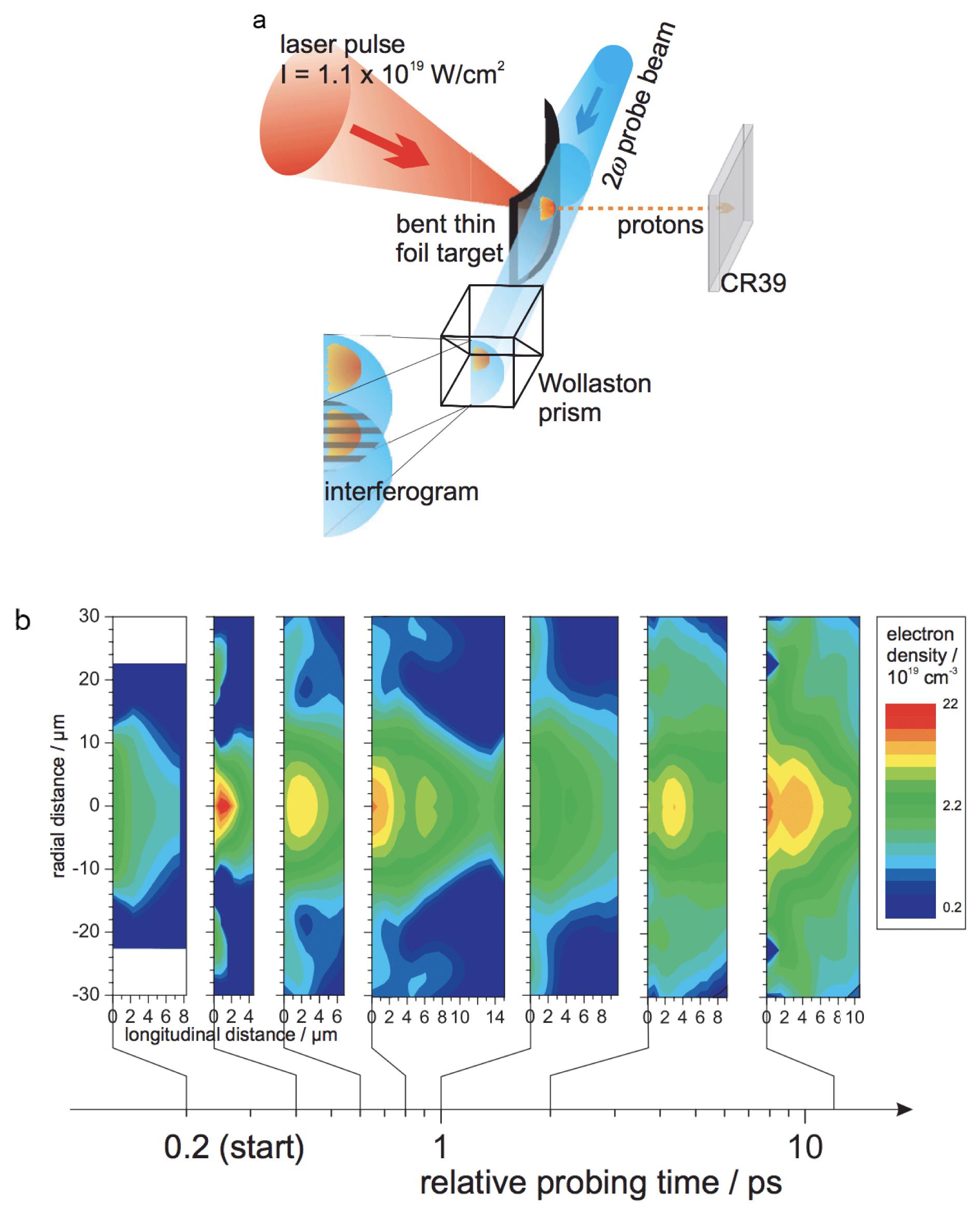
    2.1 Plasma density measurements

    The first type of measurement was presented in Refs. [24]: an all-optical diagnostic method, based on interferometry, was employed to directly measure the evolution of the hot-electron distribution driving the ion beam acceleration in the TNSA regime, adopting thin foils as targets, as shown in Figure 1. The available parameters retrieved, determining the subsequent ion acceleration, are the hot-electron density near the surface, with the temperature distribution and the conversion efficiency from laser pulse energy into hot electrons.

    2.2 Probing the quasi-static magnetic fields in plasma

    The second type of measurement was presented in Refs. [25, 26]: they detected ultra-short (picosecond regime), multi-megagauss magnetic pulses generated in a TNSA process. This diagnostic, shown in Figures 2(a) and 2(b), consisted in a pump-and-probe technique providing a complete (that is, temporal and spatial) map of these fields. The probe pulse, normally incident on target, undergoes a polarization state change induced by the magnetic field in the plasma; large and easily measurable ellipticity changes were noticed. The field evolution was obtained with high resolution both temporally (order of the pulse length) and spatially (few $\unicode[STIX]{x03BC}\text{m}$). Instead of probing the “dc” magnetic fields, similar measurements can be performed for the emitted electric field, as shown by Ref. [17]. Figure 3 shows how intense electric radiation in the THz regime is recorded behind a thin target interacting with an ultra-short (high-contrast) laser pulse. The efficient THz emission can be attributed to the hot-electron beam acceleration by the target sheath E-field. In Ref. [17] a single-shot THz time-domain spectroscopy system (TDS) with direct spatial encoding pump–probe EOS[33] (providing a ${\sim}10~\text{ps}$ time window with around 25 fs temporal resolution) was studied. Its simplicity and robustness made the technique ideal for real-time relativistic electron beam characterization. In addition, they used a Golay cell, coupled with a polyethylene polarizer, in measuring its energy and polarization, to calibrate the peak THz field on the EO crystal.

    2.3 Electromagnetic pulse detection

    A target irradiated with a high-power laser pulse blows off a large amount of charge and, in turn, the target itself emits EMPs, owing to the high return current flowing to the ground through the target holder[34]. Generally, the interaction chamber can be seen as a resonant cavity in which different modes of EMP oscillate for hundreds of nanoseconds, until the EMP is transmitted outside – for example, through the chamber glass windows – and EM waves are attenuated. However, due to the effects of small-scale structures in the target chamber, as well as of equipment inside the chamber, such as the motorized stages, cameras and other detectors, there is a shift in the ideal chamber resonant frequency[35]. The basic EMP diagnostic tool is represented by the Moebius loop antenna, typically made from solid coaxial copper cable, coupled with an electronic oscilloscope, able to measure a wide range of frequencies, up to the GHz level. As shown in Figure 4, a twist in the loop is present, which doubles the effective loop area and makes it insensitive to charged particles and ionizing radiation[36]. The two outputs are added using a matching unit to give a signal proportional to the rate of change of magnetic field. Apart from this kind of conductive antenna, recently also a dielectric electro-optic-based probe has been employed for EMP detection in an experiment with a nanosecond-long laser[23]. In particular, measurements of external electric fields have been performed by detecting the change of polarization state, induced by the electro-optic effect, of a continuous-wave laser probe beam with $\unicode[STIX]{x1D706}_{p}=1550~\text{nm}$ and circular polarization, propagating in a ${<}111>$-cut $\text{Bi}_{12}\text{SiO}_{20}$ (BSO) 5 mm thick crystal.

    2.4 Escaping particle tracking

    Other types of measurement presented here regard tracking of the escaping particles: electrons, protons, ions and photons.

    2.4.1 Magnetic spectrometer

    The first measurements of electrons produced by the interaction between an ultra-short, high-intensity laser and a solid target were presented in 1996 by Ref. [37]. The implemented diagnostic, shown in Figure 5(a), was a simple charged particle energy spectrometer, working in the range 0.4–3 MeV, composed of a pair of permanent magnets producing a uniform magnetic field $(B=1700~\text{G})$, installed along two different directions, $0^{\circ }$ and $22^{\circ }$, respectively. In this way, the electron energy spectrum was detected for different laser intensities, as reported in Figure 5(b).

    The use of a dipole spectrometer allows easy detection of charged particles and can resolve their energy spectrum. Nevertheless, there are some drawbacks: in absence of a collimator, the divergence and transverse beam size can affect this measurement; at the same time, the X-rays and $\unicode[STIX]{x03B3}$-rays produce a background on the scintillator used to track the bent particles, which can be a source of systematic error.

    2.4.2 Faraday cup

    In a laser–target environment, the Faraday cup can be adopted to detect high-energy charged particles as a real-time detector based on the time-of-flight (TOF) technique. The TOF spectrum results from a time-resolved voltage amplitude measurement, induced by charged particles impinging the Faraday cup.

    Faraday cup arrays are designed to cover different observation angles, with the normal direction to the target as reference, as shown in Figure 6(a). The diagnostic allows measurement of the two-dimensional spatial ion current density distribution and the ability to show its time evolution through TOF measurements, which is not achievable with a standard diagnostic such as laser optical interferometry. This is a unique method for two-dimensional measurements of ion currents from laser-generated plasmas, as shown in Figure 6(b).

    As mentioned, the detector is used as an ion collector in an array covering the entire emission cone and is capable of detecting high currents when it is placed in a range of few tens of centimeters from the interaction point. In common with other diagnostics, the main disadvantage is that, because of the detector position close to the interaction point, large EMPs exist and can disturb the measurements if not accurately identified and de-embedded.

    2.4.3 Radiochromic film

    Measurements of ion species parameters, such as divergence, emittance, spatial and energy resolved distribution, are of primary interest. During the interaction between powerful laser systems and targets, significant EMPs can be generated. Because of these, sensitive electronics close to the interaction point is not reliable; in contrast, film detection has been demonstrated not to be sensitive to EMPs, but electrons and X-rays can cause a signal background (easily identifiable).

    The simplest setup[38] consists in employing radiochromic film (RCF) layers acting as an energy filter. In general, particles penetrating one or more layers of the film detector deposit energy, thus the two-dimensional particle distribution can be obtained. Moreover, each film records the deposited energy, so an energy-resolved measurement (referred to as radiochromic film imaging spectroscopy) is possible. Low-energy protons are stopped in the initial film layers, whereas the most energetic penetrate and are stopped successively in the stack, as shown in Figure 7. The energy and spatially resolved proton distribution obtained from the film stack complete the beam reconstruction. Together with RCF, the use of activated materials for proton imaging has been attempted to observe global beam structures, showing positive results[39]. Moreover, Ref. [40] used silver and copper foils for energy filtering within an RCF stack. Silver foils were used to reduce the observed activity in order to minimize the exposure to the radioactive material. On the other hand, copper foils enabled absolute proton flux measurements, exploiting the $\text{}^{63}\text{Cu}~(\text{p},\text{n})~\text{}^{63}\text{Zn}$ reaction, decaying through $511~\text{keV}~\unicode[STIX]{x03B2}+$ emission, and measured using NaI co-incidence detectors. The energy filtering foils were placed onto Fuji image plates and left to be exposed to the radiation emitted from the decaying isotopes. It should be noted that, although the foil and RCF within the stack are positioned together, they do not sample the same energy slice. This is due to the threshold energy for generating a (p, n) reaction, typically around 4–5 MeV. In contrast, the RCF responds directly to the incoming radiation dose.

    2.4.4 Imaging plates

    Other diagnostic techniques widely adopted to determine the beam energy and profile are image plates (IPs) and scintillators, respectively. The IP is made of phosphors with phosphorescent properties which can release the stored energy in a de-excitation process. When photons or charged particles are incident on the IP, the electrons are promoted to a meta-stable state. Therefore, the energy stored can be retrieved by stimulating the excited meta-stable state by photons, and then the released energy (as light) is called photo-stimulated luminescence (PSL)[42]. On the other hand, a scintillator-based diagnostic can spatially resolve the transverse beam profile over a number of specified energy ranges. Multiple sheets of organic scintillators emitting light over different wavelengths can be placed in the beam path: the lowest-energy ions are stopped in the first sheet, while higher energies are stopped in subsequent sheets. As shown in Figure 8, the collected optical signal is imaged with a gated, intensified CCD camera recording the transverse beam profiles for two or more beam energy ranges[42]. IPs are sensitive to laser light and, therefore, should be properly protected to avoid signal losses. A simple strategy is to cover them with a thin aluminum foil stopping the laser.

    2.4.5 Thompson parabola

    Another diagnostic, based on collection of the escaping particles, employing both magnetic and electric fields to induce a deflection on their propagation, is called the Thompson parabola[4347]. As schematically shown in Figure 9, this diagnostic consists of an entrance pinhole, parallel electric $(E)$ and magnetic $(B)$ fields and a detector. The working principle is the following: ions with the same charge-to-mass ratio $(Z/M)$ will trace the same parabola in the detection plane, while the position of the particles along the trace depends on their energy; higher-energy ones result closer to the so-called zero point. This is an origin point where the line joining the source and the spectrometer’s entrance intercepts the detector plane and where neutral particles and photons coming from the source would hit the detector. Although Thompson parabolas allow one to clearly identify the ion species composing the beam population, they are sensitive to EMPs. To reduce this effect, it is possible to put it outside the vacuum chamber; otherwise specific de-embedding procedures should be carried out as well as having to take electronic precautions to eliminate EMP disturbances.

    2.4.6 Time-of-flight detector

    TOF measurements are also widely employed in laser–solid matter experiments[23, 4852], allowing fundamental time-resolved measurements for a detailed study of ion beam parameters, such as kinetic energy and total charge, as well as shot-to-shot reproducibility[48]. TOF spectra are usually composed by a broad ion peak signal (tens of nanoseconds at about one meter detection distance) following a narrow low-energy electrons peak and an X-ray flash. The latter, in turn, being the first to arrive on the detector, acts as a trigger for the measurement. In this scenario, semiconductor detectors are the ideal candidates. Indeed, the current response of such devices is proportional to the incident radiation energy released into the detector active layer; thus the photo-peak (usually consisting of the response to UV/soft-X-rays) is strongly lowered in comparison to the fast (high-energy) ion peak[48].

    Diamond semiconductors can be used as detectors sensitive to photons and to particles with energies above their band gap threshold, which makes them also insensitive to the visible background, which is quite noticeable in laser–plasma experiments. Nevertheless, specific designs have to be produced to eliminate EMPs coupling with the signal, as in Ref. [49]. On the other hand, the maximum detectable energy depends on the diamond thickness: the thicker the target, the higher the maximum energy is.

    2.4.7 $\unicode[STIX]{x03B3}$-ray detection

    Electrons are initially accelerated during the laser–plasma interaction; subsequently, they emit hard X-rays via the Bremsstrahlung process as they are stopped in solid material. Moreover, this phenomenon regulates the electron–positron pair production $(\unicode[STIX]{x03B3}\unicode[STIX]{x03B3}\rightarrow \text{e}^{-}\text{e}^{+})$ through photon pair annihilation, enhanced by using a high-$Z$ material as the target (for example, gold). Such high-energy photons will produce photo-nuclear reactions in almost all materials associated with the target assembly and vacuum chamber. Reference [53] designed a target in order to retrieve the Bremsstrahlung spectrum by measuring the TOF neutron energy spectrum associated with the photo-disintegration of deuterium: $\text{D}(\unicode[STIX]{x03B3},\text{n})\text{H}(Q=2.405~\text{MeV})$. Substantial radioactivity was measurable in the target assembly due to photo-nuclear reactions in both the gold target and the surrounding copper target holder, producing transmutation to platinum and nickel daughter isotopes. These processes are usually detected by means of thermo-luminescent dosimeters (TLDs). They can measure ionizing radiation from the intensity of visible light emitted by a crystal inside the detector when the crystal is heated. The intensity of light emitted is dependent upon the radiation exposure. The two most common types of TLDs are calcium fluoride (CaF) and lithium fluoride (LiF). The former is used to record $\unicode[STIX]{x03B3}$-ray exposure, and the latter for gamma and neutron exposure (indirectly, using the Li-6 (n,alpha) nuclear reaction).

    2.5 Other techniques

    Finally, it is worth mentioning an innovative technique concerning the temporal measurement of proton bursts produced from laser–solid target interactions[54], called the optical streaking technique[55], shown in Figure 10. Here, protons are accelerated via the TNSA mechanism using a $10~\unicode[STIX]{x03BC}\text{m}$ thick Au foil and collimated by means of a $100~\unicode[STIX]{x03BC}\text{m}$ Al slit (Figure 10(a)). Then, a transversely moving chirped laser pulse is used to encode the temporal profile of the proton burst: different frequency components traverse the irradiated region at different times (Figure 10(b)). Finally, the optical streak is obtained by using an imaging spectrometer (Figure 10(c)).

    3 EOS diagnostic for fast electron and electromagnetic pulse detection at SPARC_LAB

    In laser–plasma interaction experiments, time-integrated diagnostics are usually employed, as shown in the previous section. On the other hand, single-shot, time-resolved techniques are needed to properly investigate evolution of the phenomena. At the SPARC_LAB test facility[56], an EOS diagnostic (see Appendix A) has been installed in the FLAME laser[57] target area to study the electron emission from solid matter targets.

    Thus far, only indirect evidence of the escaping electrons has been detected. In particular, by measuring the X-ray emission by $\text{K}\unicode[STIX]{x03B1}$ spectroscopy, Bremsstrahlung radiation, interferometric measurement, and laser energy absorption[24, 5862], some time-integrated hot-electron properties – for example, charge, angular distribution and energy – have been directly measured. On the other hand, our diagnostic allowed us to perform direct and temporally resolved measurements.

    Some experimental campaigns[28, 29, 31] have been performed with the FLAME laser using the setup in Figure 11. The EOS diagnostic installed for this experiment relies on a $500~\unicode[STIX]{x03BC}\text{m}$ thick ZnTe crystal and, exploiting the spatial encoding technique[63], with the probe laser entering the crystal at an incidence angle $\unicode[STIX]{x1D703}_{i}\approx 28^{\circ }$, the temporal charge profile of the emitted electrons is encoded along the transverse profile of the probe laser. Since the probe diameter on the crystal is $d_{L}\approx 6~\text{mm}$, the time window provided by our diagnostic is $\unicode[STIX]{x0394}t=(d_{L}/c)\sin \unicode[STIX]{x1D703}_{i}\approx 10~\text{ps}$, where $c$ is the vacuum speed of light. Moreover, in our experimental conditions, the temporal resolution is about 100 fs. Downstream of the ZnTe crystal, as shown in Figure 11, a polarizer is set to retrieve the electric field actually encoded into the ‘EOS-probe’ signal. The polarizer is rotated $90^{\circ }$ with respect to the input laser polarization – that is, there is no light transmitted in the absence of an EO-induced phase retardation. It is able to convert the probe polarization modulation into intensity modulation. The diagnostic signal can be detected simply using a CCD camera.

    Moreover, our EOS diagnostic is also suitable to work as a TOF monitor[63, 64]. Indeed, by measuring the relative delay with respect to the reference time, the particle TOF being $\unicode[STIX]{x0394}t_{\text{TOF}}$, we can calculate the bunch velocity as $v=d/\unicode[STIX]{x0394}t_{\text{TOF}}$ and its energy as $E=\unicode[STIX]{x1D6FE}m_{e}$, where $\unicode[STIX]{x1D6FE}=1/\sqrt{1-(v/c)^{2}}$ is the relativistic Lorentz factor, $c$ is the speed of light and $m_{e}$ is the electron rest mass in eV units. Unlike conventional time-integrated techniques (for example, magnetic spectrometer), this method is able to provide energy measurements resolved in time (see Figure 12). In addition, the electric field generated by the bunch, inducing the electro-optic effect, is proportional to its charge. Therefore, the latter can be estimated from the signal intensity, making our EOS diagnostic act as a temporally resolved charge measurement with femtosecond resolution.

    To summarize, our EOS-based diagnostic allows relativistic fast electron charge and mean energy time-resolved measurements, as well as providing the temporal length of the electron bunch. To be more precise, our diagnostic can detect any external electric field whose strength is high enough to induce a birefringence in the EO crystal.

    In the following, we will treat two examples of experiments performed at SPARC_LAB: one devoted to fast electron characterization, the other for EMP detection.

    3.1 Experimental detection of fast electrons

    By means of the setup depicted in Figure 11, we were able to detect the fast electrons emitted during the interaction between the FLAME laser and a solid matter target. Indeed, since the ZnTe crystal is installed 1 mm downstream of the target, in order to avoid particles hitting the crystal, it means that, from the probe laser point of view, there is no difference whether the electron bunch has a small or large transverse radius, since the distance of the observer is larger. This distance being much larger than the Debye length ${\sim}1~\unicode[STIX]{x03BC}\text{m}$ in our experimental conditions, only the highly energetic ejected electrons escaping the potential barrier are able to reach our diagnostic. The high-resolution EOS diagnostic technique allows us to operate on the same timescale as the process, determined by the temporal duration of the main laser[22, 65]. Figure 13 explains the electric field encoding process: the signal detected by a CCD camera comes from the temporal and spatial overlap between the probe laser and the local induced birefringence. The EOS response is mainly affected by the bunch current (charge per unit time) and mean energy, while it is not affected by the energy spectrum, and therefore its distribution. It means that the signal shape, duration and strength are actually determined by the average energy of the whole electron distribution, because the low/high-energy tails in the spectrum represent the minority of the entire charge; that is, the electrons in that range of energies are too few to contribute to the development of the EOS signal. Previous reports regarding ion acceleration by lasers have demonstrated a significant energy enhancement of the accelerated ions when structured targets[6668] were employed instead of conventional targets in the TNSA scheme such as thin aluminum foils. During the laser-sharp target interaction, a higher quantity of electrons escape the target, building up a stronger potential well, which subsequently accelerates ions to higher energies. Proving this conjecture needs a direct time-resolved measurement of the escaping electrons. With this aim, we have tested different target shapes: a $10~\unicode[STIX]{x03BC}\text{m}$ thick aluminum foil, a wedged shape of stainless steel razor blade and a tip shape of a needle. Measuring the amount of charge and energy of the escaping electrons by means of the EOS detector, as explained before, provides the required evidence for the field-enhancement conjecture, summarized in Figure 14.

    For the planar foil target, as in Figure 14(a), a first emitted bunch with 1.2 nC charge and 7 MeV energy is followed (delayed by about 1.5 ps) by a second broadened structure carrying more particles (about 3 nC) but that is less energetic (about 1 MeV).

    The signal coming from the wedged target, as in Figure 14(b), shows a similar structure: the first bunch carries a larger amount of electrons (2 nC) with the same energy (7 MeV), while the second one is strongly reduced to 0.3 nC and delayed by about 2 ps. Figure 14(c) shows data captured from the tip target: the interaction with the laser produced a much larger number of fast electrons (about 7 nC), carrying also higher energies (about 12 MeV). Direct evidence of charge and energy boosts when using sharp tips can be extrapolated. Moreover, the presence of a second smaller bunch (B2) carrying about 3 nC charge can possibly be attributed to this target shape[28].

    3.2 EMP detection

    The interaction between an ultra-intense laser and a solid target also produces a huge number of EMPs. Besides the possibility to detect fast electrons, our EOS diagnostic has allowed us to reveal such EMPs. Figure 15 shows the resulting encoding process as detected by the CCD camera placed at the end of probe laser path. By means of the delay line installed along the probe laser path, it is possible to reproduce the temporal evolution of the pulses emitted by the target.

    Figure 16 shows the temporal evolution of the pulses emitted by the target, moving the delay line installed along the probe laser path by steps of 2.5 ps. Indeed, while the probe laser is delayed with respect to the interaction laser, the resulting signal moves towards the left and its amplitude decreases[31]. From this timeline, the dynamics of the target charging process can be deduced[31]. From the horizontal size of the detected signals, the charge spreading velocity or, similarly, the velocity at which the antenna emitting area grows with time, can be retrieved. We calculate a charge spreading velocity of $(0.94\,\pm \,0.03)c$, in agreement with some previous works[18, 19, 69], where $c$ is the light velocity in vacuum. Indeed, since a larger emitting area produces wider EM radiation, its radial extent is directly proportional to the horizontal size of the detected signal; meanwhile, the signal thickness is directly proportional to the average duration of the detected radiation, which, for the signals reported in Figure 16, is $6\pm 1~\text{ps}$. Furthermore, its peak value of the electric field has been found equal to 0.8 MV/m on our EOS crystal, corresponding to approximately 0.6 TV/m on target, as confirmed by particle-in-cell (PIC) simulations[31]. In addition, this field value allows only electrons with energies higher than 3 MeV to escape, in agreement with our measurements[31].

    4 Conclusions

    In conclusion, this paper provides a review regarding the different diagnostics employed in laser–solid target interaction experiments related to electron, proton and ion acceleration. Finally, we present our experimental study regarding the development of single-shot temporal diagnostics based on EOS employed for fast electron and EMP detection at the femtosecond scale. In contrast to the reviewed diagnostics, which are mostly time-integrated, our diagnostic provides single-shot, time-resolved measurements of relativistic fast electrons in terms of charge, mean energy and temporal length. In particular, nanocoulomb charged beams have been detected with multi-MeV mean energy and temporal duration ${\sim}1~\text{ps}$ FWHM. Moreover, it allowed us to observe the temporal evolution of the EMPs emitted during this kind of interaction. The fields present a temporal duration of a few picoseconds and a peak electric field amplitude ${\sim}0.6~\text{TV}/\text{m}$ on target. The values obtained are in good agreement with PIC simulations[31]. This innovative diagnostic enables discrimination between the signal carried by the fast electrons and the emitted wave generated by currents in the target. Our studies open the way to perform new time-resolved experiments aimed at reaching a deeper understanding of the phenomena involved in laser–matter interaction experiments.

    References

    [1] D. Strickland, G. Mourou. Opt. Commun., 56, 219(1985).

    [2] B. A. Remington, D. Arnett, R. P. Drake, H. Takabe. Science, 284, 1488(1999).

    [3] M. Roth, T. E. Cowan, M. H. Key, S. P. Hatchett, C. Brown, W. Fountain, J. Johnson, D. M. Pennington, R. A. Snavely, S. C. Wilks, K. Yasuike, H. Ruhl, F. Pegoraro, S. V. Bulanov, E. M. Campbell, M. D. Perry, H. Powell. Phys. Rev. Lett., 86, 436(2001).

    [4] T. Bartal, M. E. Foord, C. Bellei, M. H. Key, K. A. Flippo, S. A. Gaillard, D. T. Offermann, P. K. Patel, L. C. Jarrott, D. P. Higginson, M. Roth, A. Otten, D. Kraus, R. B. Stephens, H. S. McLean, E. M. Giraldez, M. S. Wei, D. C. Gautier, F. N. Beg. Nat. Phys., 8, 139(2012).

    [5] K. W. D. Ledingham, W. Galster. New J. Phys., 12(2010).

    [6] E. L. Clark, K. Krushelnick, M. Zepf, F. N. Beg, M. Tatarakis, A. Machacek, M. I. K. Santala, I. Watts, P. A. Norreys, A. E. Dangor. Phys. Rev. Lett., 85, 1654(2000).

    [7] R. A. Snavely, M. H. Key, S. P. Hatchett, T. E. Cowan, M. Roth, T. W. Phillips, M. A. Stoyer, E. A. Henry, T. C. Sangster, M. S. Singh, S. C. Wilks, A. MacKinnon, A. Offenberger, D. M. Pennington, K. Yasuike, A. B. Langdon, B. F. Lasinski, J. Johnson, M. D. Perry, E. M. Campbell. Phys. Rev. Lett., 85, 2945(2000).

    [8] A. J. Mackinnon, Y. Sentoku, P. K. Patel, D. W. Price, S. Hatchett, M. H. Key, C. Andersen, R. Snavely, R. R. Freeman. Phys. Rev. Lett., 88(2002).

    [9] A. G. Krygier, D. W. Schumacher, R. R. Freeman. Phys. Plasmas, 21(2014).

    [10] A. Macchi, M. Borghesi, M. Passoni. Rev. Mod. Phys., 85, 751(2013).

    [11] J. Badziak, S. Głowacz, S. Jabłoński, P. Parys, J. Wołowski, H. Hora, J. Krása, L. Láska, K. Rohlena. Plasma Phys. Control. Fusion, 46(2004).

    [12] J.-L. Dubois, F. Lubrano-Lavaderci, D. Raffestin, J. Ribolzi, J. Gazave, A. Compant La Fontaine, E. d’Humières, S. Hulin, Ph. Nicolaï, A. Poyé, V. T. Tikhonchuk. Phys. Rev. E, 89(2014).

    [13] H. Hamster, A. Sullivan, S. Gordon, W. White, R. W. Falcone. Phys. Rev. Lett., 71, 2725(1993).

    [14] M. J. Mead, D. Neely, J. Gauoin, R. Heathcote, P. Patel. Rev. Sci. Instrum., 75, 4225(2004).

    [15] A. Poyé, J.-L. Dubois, F. Lubrano-Lavaderci, E. d’Humières, M. Bardon, S. Hulin, M. Bailly-Grandvaux, J. Ribolzi, D. Raffestin, J. J. Santos, Ph. Nicolaï, V. Tikhonchuk. Phys. Rev. E, 92(2015).

    [16] A. Gopal, S. Herzer, A. Schmidt, P. Singh, A. Reinhard, W. Ziegler, D. Brömmel, A. Karmakar, P. Gibbon, U. Dillner, T. May, H.-G. Meyer, G. G. Paulus. Phys. Rev. Lett., 111(2013).

    [17] Z. Jin, H. B. Zhuo, T. Nakazawa, J. H. Shin, S. Wakamatsu, N. Yugami, T. Hosokai, D. B. Zou, M. Y. Yu, Z. M. Sheng, R. Kodama. Phys. Rev. E, 94(2016).

    [18] S. Kar, H. Ahmed, R. Prasad, M. Cerchez, S. Brauckmann, B. Aurand, G. Cantono, P. Hadjisolomou, C. L. S. Lewis, A. Macchi, G. Nersisyan, A. P. L. Robinson, A. M. Schroer, M. Swantusch, M. Zepf, O. Willi, M. Borghesi. Nat. Commun., 7(2016).

    [19] K. Quinn, P. A. Wilson, C. A. Cecchetti, B. Ramakrishna, L. Romagnani, G. Sarri, L. Lancia, J. Fuchs, A. Pipahl, T. Toncian, O. Willi, R. J. Clarke, D. Neely, M. Notley, P. Gallegos, D. C. Carroll, M. N. Quinn, X. H. Yuan, P. McKenna, T. V. Liseykina, A. Macchi, M. Borghesi. Phys. Rev. Lett., 102(2009).

    [20] S. Tokita, S. Sakabe, T. Nagashima, M. Hashida, S. Inoue. Sci. Rep., 5, 8268(2015).

    [21] C. G. Brown, A. Throop, D. Eder, J. Kimbrough. J. Phys.: Conf. Ser., 112(2008).

    [22] A. Poyé, S. Hulin, M. Bailly-Grandvaux, J.-L. Dubois, J. Ribolzi, D. Raffestin, M. Bardon, F. Lubrano-Lavaderci, E. d’Humières, J. J. Santos, Ph. Nicolaï, V. Tikhonchuk. Phys. Rev. E, 91(2015).

    [23] F. Consoli, R. De Angelis, L. Duvillaret, P. L. Andreoli, M. Cipriani, G. Cristofari, G. Di Giorgio, F. Ingenito, C. Verona. Sci. Rep., 6(2016).

    [24] O. Jäckel, J. Polz, S. M. Pfotenhauer, H. P. Schlenvoigt, H. Schwoerer, M. C. Kaluza. New J. Phys., 12(2010).

    [25] A. S. Sandhu, A. K. Dharmadhikari, P. P. Rajeev, G. R. Kumar, S. Sengupta, A. Das, P. K. Kaw. Phys. Rev. Lett., 89(2002).

    [26] G. Chatterjee, P. K. Singh, A. Adak, A. D. Lad, G. R. Kumar. Rev. Sci. Instrum., 85(2014).

    [27] H. B. Zhuo, S. J. Zhang, X. H. Li, H. Y. Zhou, X. Z. Li, D. B. Zou, M. Y. Yu, H. C. Wu, Z. M. Sheng, C. T. Zhou. Phys. Rev. E, 95(2017).

    [28] R. Pompili, M. P. Anania, F. Bisesto, M. Botton, M. Castellano, E. Chiadroni, A. Cianchi, A. Curcio, M. Ferrario, M. Galletti, Z. Henis, M. Petrarca, E. Schleifer, A. Zigler. Sci. Rep., 6(2016).

    [29] R. Pompili, M. P. Anania, F. Bisesto, M. Botton, M. Castellano, E. Chiadroni, A. Cianchi, A. Curcio, M. Ferrario, M. Galletti, Z. Henis, M. Petrarca, E. Schleifer, A. Zigler. Opt. Express, 24, 29512(2016).

    [30] F. Bisesto, M. P. Anania, M. Botton, E. Chiadroni, A. Cianchi, A. Curcio, M. Ferrario, M. Galletti, R. Pompili, E. Schleifer, A. Zigler. Quantum Beam Sci., 1, 13(2017).

    [31] R. Pompili, M. P. Anania, F. Bisesto, M. Botton, E. Chiadroni, A. Cianchi, A. Curcio, M. Ferrario, M. Galletti, Z. Henis, M. Petrarca, E. Schleifer, A. Zigler. Sci. Rep., 8, 3243(2018).

    [32] I. Wilke, A. M. MacLeod, W. A. Gillespie, G. Berden, G. M. H. Knippels, A. F. G. Van Der Meer. Phys. Rev. Lett., 88(2002).

    [33] K. Y. Kim, B. Yellampalle, A. J. Taylor, G. Rodriguez, J. H. Glownia. Opt. Lett., 32, 1968(2007).

    [34] M. De Marco, J. Krása, J. Cikhardt, M. Pfeifer, E. Krouskỳ, D. Margarone, H. Ahmed, M. Borghesi, S. Kar, L. Giuffrida, R. Vrana, A. Velyhan, J. Limpouch, G. Korn, S. Weber, L. Velardi, D. Delle Side, V. Nassisi, J. Ullschmied. J. Instrum., 11(2016).

    [35] M. De Marco, M. Pfeifer, E. Krousky, J. Krasa, J. Cikhardt, D. Klir, V. Nassisi. J. Phys.: Conf. Ser., 508(2014).

    [36] P. H. Duncan. IEEE Trans. Electromagn. Compat., EMC‐16, 83(1974).

    [37] G. Malka, J. L. Miquel. Phys. Rev. Lett., 77, 75(1996).

    [38] A. J. Mackinnon, M. Borghesi, S. Hatchett, M. H. Key, P. K. Patel, H. Campbell, A. Schiavi, R. Snavely, S. C. Wilks, O. Willi. Phys. Rev. Lett., 86, 1769(2001).

    [39] P. McKenna, K. W. D. Ledingham, L. Robson. Lasers and Nuclei, 91(2006).

    [40] R. J. Clarke, P. T. Simpson, S. Kar, J. S. Green, C. Bellei, D. C. Carroll, B. Dromey, S. Kneip, K. Markey, P. McKenna, W. Murphy, S. Nagel, L. Willingale, M. Zepf. Nucl. Instrum. Methods Phys. Res. A, 585, 117(2008).

    [41] P. R. Bolton, M. Borghesi, C. Brenner, D. C. Carroll, C. De Martinis, F. Fiorini, A. Flacco, V. Floquet, J. Fuchs, P. Gallegos, D. Giove, J. S. Green, S. Green, B. Jones, D. Kirby, P. McKenna, D. Neely, F. Nuesslin, R. Prasad, S. Reinhardt, M. Roth, U. Schramm, G. G. Scott, S. Ter-Avetisyan, M. Tolley, G. Turchetti, J. J. Wilkens. Phys. Medica, 30, 255(2014).

    [42] H. Schwoerer, S. Pfotenhauer, O. Jäckel, K.-U. Amthor, B. Liesfeld, W. Ziegler, R. Sauerbrey, K. W. D. Ledingham, T. Esirkepov. Nature, 439, 445(2006).

    [43] K. Harres, M. Schollmeier, E. Brambrink, P. Audebert, A. Blažević, K. Flippo, D. C. Gautier, M. Geißel, B. M. Hegelich, F. Nürnberg, J. Schreiber, H. Wahl, M. Roth. Rev. Sci. Instrum., 79(2008).

    [44] D. Jung, R. Hörlein, D. Kiefer, S. Letzring, D. C. Gautier, U. Schramm, C. Hübsch, R. Öhm, B. J. Albright, J. C. Fernandez, D. Habs, B. M. Hegelich. Rev. Sci. Instrum., 82(2011).

    [45] L. Torrisi, M. Cutroneo, L. Andò, J. Ullschmied. Phys. Plasmas, 20(2013).

    [46] F. Consoli, R. De Angelis, P. Andreoli, G. Cristofari, G. Di Giorgio, A. Bonasera, M. Barbui, M. Mazzocco, W. Bang, G. Dyer, H. Quevedo, K. Hagel, K. Schmidt, E. Gaul, T. Borger, A. Bernstein, M. Martinez, M. Donovan, M. Barbarino, S. Kimura, J. Sura, J. Natowitz, T. Ditmire. Nucl. Instrum. Methods Phys. Res. A, 720, 149(2013).

    [47] A. Alejo, D. Gwynne, D. Doria, H. Ahmed, D. C. Carroll, R. J. Clarke, D. Neely, G. G. Scott, M. Borghesi, S. Kar. J. Instrum., 11(2016).

    [48] D. Margarone, J. Krása, L. Giuffrida, A. Picciotto, L. Torrisi, T. Nowak, P. Musumeci, A. Velyhan, J. Prokpek, L. Láska, T. Mocek, J. Ullschmied, B. Rus. J. Appl. Phys., 109(2011).

    [49] R. De Angelis, F. Consoli, C. Verona, G. Di Giorgio, P. Andreoli, G. Cristofari, M. Cipriani, F. Ingenito, M. Marinelli, G. Verona-Rinati. J. Instrum., 11(2016).

    [50] S. Busold, D. Schumacher, O. Deppert, C. Brabetz, S. Frydrych, F. Kroll, M. Joost, H. Al-Omari, A. Blažević, B. Zielbauer, I. Hofmann, V. Bagnoud, T. E. Cowan, M. Roth. Phys. Rev. ST Accel., 16(2013).

    [51] L. Gizzi, D. Giove, C. Altana, F. Brandi, P. Cirrone, G. Cristoforetti, A. Fazzi, P. Ferrara, L. Fulgentini, P. Koester, L. Labate, G. Lanzalone, P. Londrillo, D. Mascali, A. Muoio, D. Palla, F. Schillaci, S. Sinigardi, S. Tudisco, G. Turchetti. Appl. Sci., 7, 984(2017).

    [52] F. Bisesto, M. Galletti, M. P. Anania, F. Massimo, R. Pompili, M. Botton, A. Zigler, F. Consoli, M. Salvadori, P. Andreoli, C. Verona. High Power Laser Sci. Eng., 7(2019).

    [53] M. D. Perry, J. A. Sefcik, T. Cowan, S. Hatchett, A. Hunt, M. Moran, D. Pennington, R. Snavely, S. C. Wilks. Rev. Sci. Instrum., 70, 265(1999).

    [54] B. Dromey, M. Coughlan, L. Senje, M. Taylor, S. Kuschel, B. Villagomez-Bernabe, R. Stefanuik, G. Nersisyan, L. Stella, J. Kohanoff, M. Borghesi, F. Currell, D. Riley, D. Jung, C.-G. Wahlström, C. L. S. Lewis, M. Zepf. Nat. Commun., 7(2016).

    [55] D. Polli, D. Brida, S. Mukamel, G. Lanzani, G. Cerullo. Phys. Rev. A, 82(2010).

    [56] M. Ferrario, D. Alesini, M. Anania, A. Bacci, M. Bellaveglia, O. Bogdanov, R. Boni, M. Castellano, E. Chiadroni, A. Cianchi, S. B. Dabagov, C. De Martinis, D. Di Giovenale, G. Di Pirro, U. Dosselli, A. Drago, A. Esposito, R. Faccini, A. Gallo, M. Gambaccini, C. Gatti, G. Gatti, A. Ghigo, D. Giulietti, A. Ligidov, P. Londrillo, S. Lupi, A. Mostacci, E. Pace, L. Palumbo, V. Petrillo, R. Pompili, A. R. Rossi, L. Serafini, B. Spataro, P. Tomassini, G. Turchetti, C. Vaccarezza, F. Villa, G. Dattoli, E. Di Palma, L. Giannessi, A. Petralia, C. Ronsivalle, I. Spassovsky, V. Surrenti, L. Gizzi, L. Labate, T. Levato, J. V. Rau. Nucl. Instrum. Methods Phys. Res. B, 309, 183(2013).

    [57] F. G. Bisesto, M. P. Anania, M. Bellaveglia, E. Chiadroni, A. Cianchi, G. Costa, A. Curcio, D. Di Giovenale, G. Di Pirro, M. Ferrario, F. Filippi, A. Gallo, A. Marocchino, R. Pompili, A. Zigler, C. Vaccarezza. Nucl. Instrum. Methods Phys. Res. A, 909, 452(2018).

    [58] M. H. Key, M. D. Cable, T. E. Cowan, K. G. Estabrook, B. A. Hammel, S. P. Hatchett, E. A. Henry, D. E. Hinkel, J. D. Kilkenny, J. A. Koch, W. L. Kruer, A. B. Langdon, B. F. Lasinski, R. W. Lee, B. J. MacGowan, A. MacKinnon, J. D. Moody, M. J. Moran, A. A. Offenberger, D. M. Pennington, M. D. Perry, T. J. Phillips, T. C. Sangster, M. S. Singh, M. A. Stoyer, M. Tabak, G. L. Tietbohl, M. Tsukamoto, K. Wharton, S. C. Wilks. Phys. Plasmas, 5, 1966(1998).

    [59] P. M. Nilson, J. R. Davies, W. Theobald, P. A. Jaanimagi, C. Mileham, R. K. Jungquist, C. Stoeckl, I. A. Begishev, A. A. Solodov, J. F. Myatt, J. D. Zuegel, T. C. Sangster, R. Betti, D. D. Meyerhofer. Phys. Rev. Lett., 108(2012).

    [60] Y. Ping, R. Shepherd, B. F. Lasinski, M. Tabak, H. Chen, H. K. Chung, K. B. Fournier, S. B. Hansen, A. Kemp, D. A. Liedahl, K. Widmann, S. C. Wilks, W. Rozmus, M. Sherlock. Phys. Rev. Lett., 100(2008).

    [61] M. I. K. Santala, M. Zepf, I. Watts, F. N. Beg, E. Clark, M. Tatarakis, K. Krushelnick, A. E. Dangor, T. McCanny, I. Spencer, R. P. Singhal, K. W. D. Ledingham, S. C. Wilks, A. C. Machacek, J. S. Wark, R. Allott, R. J. Clarke, P. A. Norreys. Phys. Rev. Lett., 84, 1459(2000).

    [62] H. Chen, R. Shepherd, H. K. Chung, A. Kemp, S. B. Hansen, S. C. Wilks, Y. Ping, K. Widmann, K. B. Fournier, G. Dyer, A. Faenov, T. Pikuz, P. Beiersdorfer. Phys. Rev. E, 76(2007).

    [63] A. L. Cavalieri, D. M. Fritz, S. H. Lee, P. H. Bucksbaum, D. A. Reis, J. Rudati, D. M. Mills, P. H. Fuoss, G. B. Stephenson, C. C. Kao, D. P. Siddons, D. P. Lowney, A. G. MacPhee, D. Weinstein, R. W. Falcone, R. Pahl, J. Als-Nielsen, C. Blome, S. Dusterer, R. Ischebeck, H. Schlarb, H. Schulte-Schrepping, Th. Tschentscher, J. Schneider, O. Hignette, F. Sette, K. Sokolowski-Tinten, H. N. Chapman, R. W. Lee, T. N. Hansen, O. Synnergren, J. Larsson, S. Techert, J. Sheppard, J. S. Wark, M. Bergh, C. Caleman, G. Huldt, D. van der Spoel, N. Timneanu, J. Hajdu, R. A. Akre, E. Bong, P. Emma, P. Krejcik, J. Arthur, S. Brennan, K. J. Gaffney, A. M. Lindenberg, K. Luening, J. B. Hastings. Phys. Rev. Lett., 94(2005).

    [64] R. Pompili, M. P. Anania, M. Bellaveglia, A. Biagioni, G. Castorina, E. Chiadroni, A. Cianchi, M. Croia, D. Di Giovenale, M. Ferrario, F. Filippi, A. Gallo, G. Gatti, F. Giorgianni, A. Giribono, W. Li, S. Lupi, A. Mostacci, M. Petrarca, L. Piersanti, G. Di Pirro, S. Romeo, J. Scifo, V. Shpakov, C. Vaccarezza, F. Villa. New J. Phys., 18(2016).

    [65] J. Fuchs, P. Antici, E. d’Humières, E. Lefebvre, M. Borghesi, E. Brambrink, C. A. Cecchetti, M. Kaluza, V. Malka, M. Manclossi, S. Meyroneinc, P. Mora, J. Schreiber, T. Toncian, H. Pépin, P. Audebert. Nat. Phys., 2, 48(2006).

    [66] A. Zigler, S. Eisenman, M. Botton, E. Nahum, E. Schleifer, A. Baspaly, I. Pomerantz, F. Abicht, J. Branzel, G. Priebe, S. Steinke, A. Andreev, M. Schnuerer, W. Sandner, D. Gordon, P. Sprangle, K. W. D. Ledingham. Phys. Rev. Lett., 110(2013).

    [67] A. Zigler, T. Palchan, N. Bruner, E. Schleifer, S. Eisenmann, M. Botton, Z. Henis, S. A. Pikuz, A. Y. Faenov, D. Gordon, P. Sprangle. Phys. Rev. Lett., 106(2011).

    [68] D. Margarone, O. Klimo, I. J. Kim, J. Prokupek, J. Limpouch, T. M. Jeong, T. Mocek, J. Psikal, H. T. Kim, J. Proska, K. H. Nam, L. Stolcova, I. W. Choi, S. K. Lee, J. H. Sung, T. J. Yu, G. Korn. Phys. Rev. Lett., 109(2012).

    [69] L. Romagnani, J. Fuchs, M. Borghesi, P. Antici, P. Audebert, F. Ceccherini, T. Cowan, T. Grismayer, S. Kar, A. Macchi, P. Mora, G. Pretzler, A. Schiavi, T. Toncian, O. Willi. Phys. Rev. Lett., 95(2005).

    [70] S. Casalbuoni, H. Schlarb, B. Schmidt, P. Schmüser, B. Steffen, A. Winter. Phys. Rev. ST Accel., 11(2008).

    Fabrizio Bisesto, Mario Galletti, Maria Pia Anania, Massimo Ferrario, Riccardo Pompili, Mordechai Botton, Elad Schleifer, Arie Zigler. Review on TNSA diagnostics and recent developments at SPARC_LAB[J]. High Power Laser Science and Engineering, 2019, 7(3): 03000e56
    Download Citation