Turbulence-induced beam wandering during femtosecond laser filamentation

Tao Zeng; Hui Gao; Xiaodong Sun; Weiwei Liu

doi:10.3788/COL201513.070008

Abstract

The influence of air turbulence on the transverse wandering of a single femtosecond laser filament is studied by numerical simulation. The results show that the average transverse displacement of the single filament

δ r

is proportional to the square root of turbulent structure constant and the relations between

δ r

and the propagation distance can be fit by a power function. In addition, by using an axicon as a focusing optics, the wandering of a single filament is suggested to be stronger than the free-propagation case.

Femtosecond filamentation has drawn much attention in the fields of femtosecond lasers and atmospheric science recently^[1–6]. The filamentation phenomenon contains useful physical processes, such as the dynamic interplay between the self-focusing caused by the optical Kerr effect and plasma defocusing, self-phase modulation, self-steepening, and so on^[1–4]. It has shown great value for remote sensing^[5,6], lightning control^[7,8], pulse compression^[9–11], and terahertz (THz) wave generation^[12,13].

As the femtosecond laser pulse propagates through the atmosphere, the influence of the air turbulence on the process of filamentation must be taken into consideration. The spatial wandering of a single filament due to the turbulence in air has been observed both experimentally and numerically in Ref. [14].

Spatial wandering of a filament caused by the turbulence could be crucial for applications such as remote air lasing^[15–18] and pulse self-compression^[19–24]. Nevertheless, the dependence of the beam wandering on the propagation distance and the strength of the air turbulence during the filamentation process has not been revealed yet. Clearly, this information will be quite important consideration for the aforementioned applications of the filamentation.

Sign up for Chinese Optics Letters TOC. Get the latest issue of Chinese Optics Letters delivered right to you！Sign up now

In this work, the influence of air turbulence on the transverse wandering of single filaments has been investigated by numerical simulation. The relationship between the filament deviation and the structure constant of air turbulence which determines the intensity of fluctuations of the air refractive index has been revealed. Furthermore, we explored the feasibility of using an axicon as a focusing optics to investigate the wandering of a single filament propagating through the turbulent atmosphere.

The numerical simulations were carried out based on the $2 D + 1 [A (x, y, z)]$ nonlinear wave equation^[14,25] $2 i k_{0} \frac{\partial A}{\partial z} + (\frac{\partial^{2}}{\partial x^{2}} + \frac{\partial^{2}}{\partial y^{2}}) A + 2 k_{0}^{2} Δ n A + 2 k_{0}^{2} \tilde{n} (x, y, z) A = 0,$ (1)where $A$ represents the amplitude of the light field and $k_{0}$ is the wave number of the beam with the central wavelength of 800 nm in our simulation. Term $Δ n$ includes the nonlinear refractive index induced by the optical Kerr effect ( $Δ n_{ker} = n_{2} I$ ) and the effective counteracting higher-order nonlinear refractive index of plasma defocusing effect ( $Δ n_{plasma} = - σ I^{m}$ ). The coefficient $n_{2}$ is $2 \times 10^{- 19} {cm}^{2} / W$ and $m$ is chosen to be 8^[26]. Term $σ$ is an empirical parameter which gives rise to a clamped intensity of $5 \times 10^{13} W / {cm}^{2}$ ^[25]. It is easy to see that Eq. (1) describes the propagation of a CW beam in a medium with saturable nonlinearity. It is also worth mentioning that since we focus mainly on the spatial distribution of the multiple filaments, the temporal aspects of the nonlinear propagation are not considered in Eq. (1). The validity of this kind simplification has been demonstrated by previous studies^[27,28]. Term $\tilde{n} (x, y, z)$ denotes the fluctuations of the air refractive index due to the atmosphere turbulence. In order to include the spatial fluctuations of the refractive index, we use the modified Karman spectrum which is the classical model describing the atmospheric turbulence^[29] $F_{n} (κ_{x}, κ_{y}, κ_{z}) = 0.033 C_{n}^{2} {(κ^{2} + κ_{0}^{2})}^{- \frac{11}{6}} \exp [- {(κ / κ_{m})}^{2}],$ (2)where $κ$ represents the spatial wave number and is given by $κ = κ_{x}^{2} + κ_{y}^{2} + κ_{z}^{2}$ , where $κ_{x}$ , $κ_{y}$ , and $κ_{z}$ refer to three components of κ along the $x$ , $y$ , and $z$ coordinates, respectively. Term $C_{n}^{2}$ refers to the refractive index structure constant, while $κ_{0} = 2 π / L_{0}$ and $κ_{m} = 5.92 / l_{0}$ . Terms $L_{0}$ and $l_{0}$ are the outer and inner scales of turbulence, respectively. The scale of the turbulent air refractive index fluctuations varies from the inner scale $l_{0}$ which is about 0.1–1 cm to the outer scale $L_{0}$ which can be tens of meters^[30].

Then we use the phase screen model to represent the three-dimensional refractive index fluctuations based on the aforementioned Karman spectrum. The beam propagation range is divided into several segments and the phase fluctuations spectral density of each segment $Δ z$ has the form $F_{ϕ} (κ_{x}, κ_{y}) = 2 π k_{0}^{2} Δ z F_{n} (κ_{x}, κ_{y}, 0) .$ (3)

The outer scale of turbulence is chosen to be 1 m and the inner scale equals 1 mm in our simulation. Different phase screens, which represent a cumulative phase shift of 1 m distance with different series of random numbers, can be obtained according to Eq. (3)^[30].

Then the spatial phase fluctuations are reconstructed by the summation of the Fourier harmonics of the spatial spectrum indicated by Eq. (3). The random complex 2D field of phase fluctuations $Φ_{n m}$ at the nodes of a uniform computational grid $n$ , $m$ is thus given by $ϕ_{n m} = \frac{1}{\sqrt{N M}} \sum_{p = - \frac{N}{2}}^{\frac{N}{2} - 1} \sum_{q = - \frac{M}{2}}^{\frac{M}{2} - 1} a_{p q} (ε_{p q} + i η_{p q}) \exp [i \frac{2 π}{N} (p n + q m)],$ (4)where $N$ and $M$ are the numbers of the computational nodes. Terms $ε_{p q}$ and $η_{p q}$ are statistically independent random numbers distributed uniformly over the range $[- \sqrt 3, \sqrt 3]$ , and $a_{p q}$ is determined by the spectral density of phase fluctuations as follows $a_{p q}^{2} = F_{ϕ} (p Δ k_{x}, q Δ k_{y}) Δ k_{x} Δ k_{y},$ (5)where $Δ k_{x}$ and $Δ k_{y}$ are connected with the transverse dimensions of the phase screen $L_{x}$ and $L_{y}$ , respectively, as $Δ k_{x} = \frac{2 π}{L_{x}}, Δ k_{y} = \frac{2 π}{L_{y}} .$ (6)

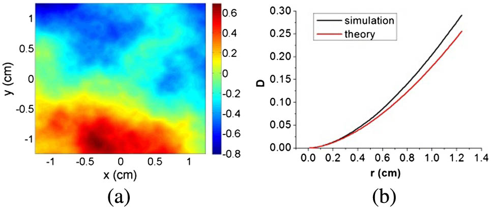
The use of additional information about the low-frequency wing of the spectrum has been proposed in many references to modify the aforementioned spectral method^[31,32]. The contribution of the low-frequency spectral component to the resulting phase screen is described by $ϕ_{n m}^{LF} = \sum_{k = 1}^{N_{k}} 3^{- k} \frac{1}{\sqrt{N M}} \sum_{p = - 3}^{2} \sum_{q = - 3}^{2} a_{p q} (ε_{p q} + i η_{p q}) \times \exp {i \frac{2 π}{N} 3^{- k} [(p + 0.5) n + (q + 0.5) m]},$ (7)where $a_{p q}^{2} = F_{ϕ} [3^{- k} (p + 0.5) Δ k_{x}, 3^{- k} (q + 0.5) Δ k_{y}] Δ k_{x} Δ k_{y}$ and $k = 1, \dots, N_{k}$ .

As an illustration, Fig. 1(a) shows a phase screen created by the superposition of two separate phase screens according to Eqs. (4) and (7) with $N_{k} = 4$ , the structure constant $C_{n}^{2} = 10^{- 13} {cm}^{- 2 / 3}$ , and the distance $Δ z = 1 m$ . Finally the fluctuations of $\tilde{n} (x, y, z)$ within the beam propagation distance of $Δ z$ can be obtained by the particular phase screen $ϕ (x, y)$ approximately as follows $\tilde{n} (x, y, z) = \frac{ϕ (x, y)}{k_{0} Δ z} .$ (8)

Figure 1.(a) Representative phase screen with structure constant $C_{n}^{2} = 10^{- 13} {cm}^{- 2 / 3}$ and distance $Δ z = 1 m$ ; (b) structure function of phase fluctuations. Black line refers to simulation result and red line corresponds to theoretical prediction.

Note that the validity of the phase screens created through the aforementioned method could be tested with reference to the theoretical phase structure function, which is written as^[29] $D (r) = 〈 {[φ (r^{'}) - φ (r^{'} + r)]}^{2} 〉 = 6.88 {(r / r_{0})}^{5 / 3},$ (9)where $r$ denotes the distance between any two points in the phase screen and $r_{0}$ represents the Fried parameter^[33]. The brackets mean the average over an ensemble phase screens, which can be calculated by using the simulated phase screen. The comparison result is shown in Fig. 1(b). The structure function of phase fluctuations shown in Fig. 1(b) as a black curve is obtained by averaging over 100 statistically independent screens^[30], while the red curve represents the outcome computed according to by the right-hand side of Eq. (8). The slight discrepancy appearing in Fig. 1(b) may come from the limited screen dimensions. Note that temporal variation of turbulence is not considered in our numerical simulation. It is reasonable since in practice the laser pulse duration is many orders of magnitudes shorter than the typical hydrodynamics time scale of turbulence.

During our work, three cases have been considered. As indicated in Fig. 2, in Case A, the turbulence exists prior to the beam collapse during the propagation. The radius of the initial CW laser beam with a Gaussian profile is 2.5 mm, while the initial laser power is chosen to be 5 times the critical power for self-focusing. The estimated self-focusing distance is about 6.55 m^[2,34]. The turbulence is introduced into the self-focusing process during the first 6-m propagation distance. The displacement of the beam center which is calculated as the centroid of the single filament spot in the transverse plane is registered at the collapse position ( $z = 6 m$ ). This process has been repeated 30 times by using different phase screens with the same turbulence structure constant $C_{n}^{2} = 6.4 \times 10^{- 13} {cm}^{- 2 / 3}$ . The distribution of the beam center positions obtained with 30 statistically independent chains of random phase screens has been displayed in Fig. 3(a). The corresponding average value of the transverse beam center displacement $〈 δ r 〉$ is about 236.1 μm.

Figure 2.Three cases of the simulation: (a) turbulence is introduced prior to filament formation; (b) turbulence is introduced after filament formation; (c) axicon is used as focusing optics.

Figure 3.Spatial displacements of a single filament center in turbulent air obtained with 30 statistically independent chains of random phase screens but the same turbulent structure constant $C_{n}^{2} = 6.4 \times 10^{- 13} {cm}^{- 2 / 3}$ for three different conditions: (a) turbulence is introduced prior to filament formation; (b) turbulence is introduced after filament formation; (c) axicon is used as focusing optics.

The same simulation process has been adopted to study Case B shown in Fig. 2. The difference between Cases B and A is that turbulence is introduced after the beam collapse distance where the plasma starts to be formed. Similarly to Case A, the filament center position has been recorded 6 m away from the beginning of the turbulence. The corresponding results are shown in Fig. 3(b). The average of the transverse displacement $〈 δ r 〉$ of the filament center under this condition reads 209.0 μm. Figures 3(a) and 3(b) imply that the effect of air turbulence on the filament pointing stability is more significant when the turbulence occurs prior to the onset of filamentation than when it takes place in the middle of the filament. It agrees with the conclusion given by Ref. [35].

It is worth mentioning that the axicon has been commonly used in the process of filamentation to elongating the filament length^[36–39]. Therefore, it would be interesting to understand the effect of turbulence when an axicon is used as the focusing optics to generate filament. The simulation scheme is illustrated in Fig. 2(c). A CW laser beam with the central wavelength of 800 nm is incident on an axicon. The power of the initial beam with a radius $R$ of 2.5 mm ( $1 / e^{2}$ ) is also 5 $P_{c r}$ . The bottom angle of the axicon $α$ was chosen to be 0.03°. Under this condition, the effective focal depth $Z_{D}$ of the laser beam focused by the axicon is 918.2 cm in air^[40,41]. In Case C, the turbulence with the same structure constant as Cases A and B is applied on the beam starting at a distance of 2.5 m from the axicon. By creating 30 sets of phase screens with different random numbers, the beam center wandering at the distance of 6 m from the beginning of the turbulence is depicted in Fig. 3(c). The average of the transverse displacement $〈 δ r 〉$ of the filament center in this case is 421.8 μm, which is obviously larger than those in the Cases A and B. The result indicates that the axicon shows no advantage as a focusing optics in suppressing the wandering of a single filament propagating through the turbulent atmosphere.

In the next step the average displacement $〈 δ r 〉$ of the single filament wandering has been investigated as a function of the turbulent structure constant $C_{n}^{2}$ varied from $10^{- 14}$ to $10^{- 12} {cm}^{- 2 / 3}$ for all three cases, which covers from standard atmospheric turbulence several meters above the ground to relative strong turbulence^[42]. The obtained results are shown in Fig. 4(a). In Cases A and B, the relations between $〈 δ r 〉$ and the square root of $C_{n}^{2}$ can be fit linearly. The slopes of the linear fitting are 29.5 and 26.2 for Cases A and B, respectively. The results present in Fig. 4(a) confirm that when using the axicon, the spatial wandering of a filament in turbulent atmosphere is even stronger than the free-propagation case. It could be understood as the following. When using an axicon, the outer rings of the created Bessel shape beam equivalently constitutes the energy reservoir of the filament located on the center propagation axis. The outer diameter of these rings is essentially many times larger than the size of the filament itself. Hence, the energy reservoir suffers strong effect of the turbulence. On the other hand, the diameter of the energy reservoir of a free-propagation filament is generally close to 1 mm, which is close to the inner diameter of the considered turbulence. As a consequence, the turbulence effect on a filament in the case of free-propagation would be weaker as compared with the case by using an axicon.

Figure 4.(a) Averaged transverse displacement of a single filament as a function of the square root of the turbulent structure constant; (b) averaged transverse displacement of a single filament versus filament length in turbulent air ( $C_{n}^{2} = 6.4 \times 10^{- 13} {cm}^{- 2 / 3}$ , solid circles) and the fitting (solid line).

In addition, the filament transverse wandering have been studied versus the propagation distance in turbulent air. The turbulent structure constant $C_{n}^{2}$ is set to be $6.4 \times 10^{- 13} {cm}^{- 2 / 3}$ . The phase screens obtained with different random numbers are inserted within the filamentation zone for every 1 m in three different cases. The filament length varied from 1 to 6 m. Thirty shots are obtained for each distance. The final result is shown in Fig. 4(b). The relations between $〈 δ r 〉$ and the filament length can be fitted by a power function $〈 δ r 〉 = a z^{b},$ (10)where $a$ is 11.37, 13.34, and 13.08 for Cases A–C, respectively. Term $b$ is 1.70, 1.54, and 1.93 for Cases A–C, respectively. The values of $b$ reflect the effect of the beam diameters on the beam wandering induced by the turbulence. In Case B, the energy reservoir has the smallest dimension. When the axicon is used in Case C, the energy reservoir occupies the largest diameter. Since for a single filament in the free-propagation case, the size of the energy reservoir is essentially constant, the beam wondering inside the filament may follow the same power function versus the propagation distance as the Case B, i.e., $b \approx 1.5$ , giving us the opportunity to estimate the beam wandering of the filaments.

In conclusion, we study the influence of air turbulence on single filament transverse wandering based on numerical simulation. During the propagation of a single filament in the turbulent atmosphere, it is revealed that the average transverse displacement $〈 δ r 〉$ of the single filament is proportional to the square root of the turbulent structure constant and the relations between $〈 δ r 〉$ and the propagation distance can be fit by a power function. Furthermore, it is demonstrated that the axicon shows no advantage as focusing optics in suppressing the wandering of a single filament propagating through the turbulent air. Our work can be valuable for optimizing the performance of remote air lasing and pulse compression assisted by femtosecond laser filamentation.

References

[1] J. Kasparian, M. Rodriguez, G. Mejean, J. Yu, E. Salmon, H. Wille, R. Bourayou, S. Frey, Y. B. Andre, A. Mysyrowicz, R. Sauerbrey, J. P. Wolf, L. Woste. Science, 301, 61(2003).

[2] A. Couairon, A. Mysyrowicz. Phys. Rep., 441, 47(2007).

[3] J. Kasparian, J. P. Wolf. Opt. Express, 16, 466(2008).

[4] S. L. Chin, H. L. Xu, Y. Cheng, Z. Z. Xu, K. Yamanouchi. Chin. Opt. Lett., 11, 013201(2013).

[5] H. L. Xu, S. L. Chin. Sensors, 11, 32(2011).

[6] J. Odhner, R. Levis. Annu. Rev. Phys. Chem., 65, 605(2014).

[7] H. Pépin, D. Comtois, F. Vidal, C. Y. Chien, A. Desparois, T. W. Johnston, J. C. Kieffer, B. La Fontaine, F. Martin, F. A. M. Rizk, C. Potvin, P. Couture, H. P. Mercure, A. Bondiou-Clergerie, P. Lalande, I. Gallimberti. Phys. Plasma, 8, 2532(2001).

[8] M. Rodriguez, R. Sauerbrey, H. Wille, L. Woste, T. Fujii, Y. B. Andre, A. Mysyrowicz, L. Klingbeil, K. Rethmeier, W. Kalkner, J. Kasparian, E. Salmon, J. Yu, J. P. Wolf. Opt. Lett., 27, 772(2002).

[9] S. Akturk, A. Couairon, M. Franco, A. Mysyrowicz. Opt. Express, 16, 17626(2008).

[10] F. Kong, Y. Jin, S. Liu, S. Chen, H. Guan, K. He, Y. Du, H. He. Chin. Opt. Lett., 11, 102302(2013).

[11] O. G. Kosareva, I. N. Murtazin, N. A. Panov, A. B. Savel’ev, V. P. Kandidov, S. L. Chin. Laser Phys. Lett., 4, 126(2007).