
[in Chinese], [in Chinese], [in Chinese], [in Chinese], [in Chinese], [in Chinese], "Numerical simulation of debris-removal trajectories on the transport mirrors in high-power laser systems," High Power Laser Sci. Eng. 3, 010000e5 (2015)
- High Power Laser Science and Engineering
- Vol. 3, Issue 1, 010000e5 (2015)
Abstract
Keywords
1. Introduction
High-power laser systems (HPLSs) are large optical instruments for high-energy physics and inertial confinement fusion. The transport mirrors of HPLSs direct light from the main amplifiers to the target and impact remarkably upon the quality of laser beams arriving at the target[
The debris on mirrors includes natural dust falls, metal fragments, and organic fibers left during operations. Numerous methods have been used to keep the optical devices clean, but to date, few experimental results have demonstrated the optical cleanliness of the whole laser facility[ using high-speed airflow generated by an air knife[
In the present study, the flow field and the removal trajectories of debris with varied types and sizes on the transport mirror are numerically investigated. A device is fabricated based on the simulation results. This device can capture and collect debris from the mirror surface online.
Sign up for High Power Laser Science and Engineering TOC. Get the latest issue of High Power Laser Science and Engineering delivered right to you!Sign up now
2. The numerical model
Computational fluid dynamics (CFD) is an important technique for investigating flow fields. With computer numerical calculation and image display, CFD can conduct numerical simulations on a system containing relevant physical phenomena, such as fluid flow and heat. Numerical analysis of the flow field with basic physical quantities (such as speed, pressure, temperature and concentration), as well as the distribution of fluid trajectory, is now a popular topic in fluid studies.
2.1. The model to be calculated
A two-dimensional (2D) model satisfies the requirements of understanding the fluid field and the trajectories of contaminant particles. The 2D model in this study included one air knife, one transport mirror and one cover (Figure
The 2D model was implemented using the business software Gambit 2.4.6, used for geometry and mesh generation, and the 20 640 quadrilateral elements were divided by quadrilateral mesh structures[ .
.
2.2. Boundary conditions and associated settings
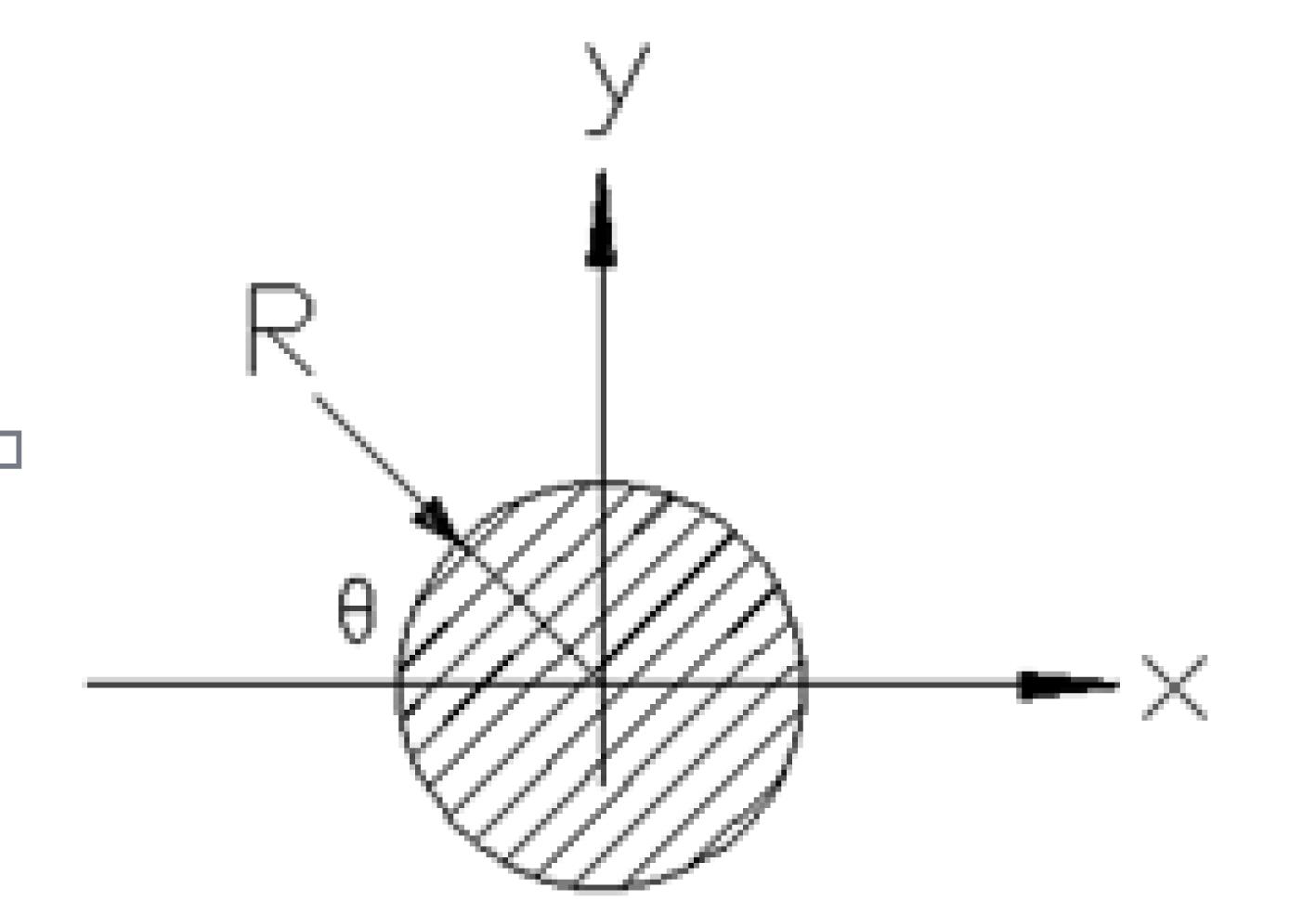
The best way to remove a particle is to blow in the direction of the  -axis, where the particle can be subjected to maximum thrust
  (Figure
  -axis). Thus, the particle is subjected to the maximum force and easily removed when the blowing surface is situated on the
  -axis. Therefore, a suitable distance
  between the up-surfaces of the transport mirror and the air knife was chosen to make the transport mirror surface close to, or coinciding with, the centerline of the airflow (Figure
  . Finally, the airflow entered the up-surface
  of the transport mirror and moved along the up-surface. After a series of experiments, a good particle removal effect was obtained when the air pressure was 9 atm and
  was 3 mm.
Boundary conditions were set as follows. The outlet of the air knife was the pressure inlet. The gage total pressure was 9 atm, the supersonic/initial gage total pressure was 7 atm, the inlet temperature was 300 K and the turbulent energy and default dissipation rates were 1.
Boundaries  ,
,  ,
,  , and
, and  were the pressure outlets.
  ,
,  ,
,  , and
, and  . The outlet temperature was 300 K. The turbulent energy and default dissipation rate were 1. The gage total pressures of boundaries
  ,
,  ,
,  and
and  were 1 atm. The gage total pressure of boundary
  was 0.8 atm.
The remaining boundaries were walls, which were non-slip walls.  ,
,  , and the length
  of the up-surface of the transport mirror was 400 mm. Dust, aluminum particles and stainless steel particles, with sizes of 10, 20, 40, and 80
  , were used as debris, and they were uniformly distributed on the surface of the transport mirror. The densities of dust, aluminum (Al) particles and stainless steel (ss) particles were 1000, 2700 and
  , respectively.
2.3. Governing equations
The basic equations of fluid analysis, turbulent flow and particle motion were used as the control equations[ model, which is an improved model of the standard turbulent model of
  . The particle motion equation was the force-balance equation in Cartesian coordinates.
3. Simulation results and discussion
3.1. Flow field
Figures  in the region near the outlet of the air knife (Figure
  . The negative pressure of outlet
  can steer flow. The air speed is
  , which approximately decreases along the
  -axis. These high speeds blow the particles away from the transport mirror.
3.2. Debris trajectories
Dust particles with four different sizes were considered. For each size, 200 dust particles were evenly placed on the transport mirror up-surface  from the left to the right, and a numerical simulation was performed based on the numerical model and settings stated in Section
  , respectively. Each curve represents one type of movement tendency of some particles. There are a total of three kinds of movement trends: type 1, type 2 and type 3. Besides this, curves of type 1 in Figure
The simulation results demonstrate that the motion displacements of the majority of the particles are small in the vertical direction, almost slipping along the upper surface of the mirror (type 2). The  -coordinate of the upper mirror surface is 2 mm; thus the minimum value of
  in Figure
The  values of particles increase rapidly, decrease, then increase along the path, and finally decrease (type 1). This event is due to the fact that the region of the 10 particles instantly becomes a negative pressure zone when the air knife is blowing. Then, turbulences (Figure
  values, the pneumatic forces weaken, gravity gradually dominates, and the velocities decrease to zero. During this period, the
  values reach maximum. Then, the particles move along the negative direction of the
  -axis, the
  values decrease, and the vortices are strengthened. The velocities of the particles along the negative direction of the
  -axis are gradually reduced to zero when the pneumatic forces are large enough to overcome gravity. Then, the velocity direction reverses, and the
  values increase. Gradually, the
  values decrease because the negative pressure of the outlet
  can steer flow.
With the increase in particle sizes, the numbers of particles of type 3 that begin to reach the maximum  values, hit the mirror surface and finally rebound off the surface also increase. This phenomenon is due to insufficient pneumatic forces to overcome the additional gravity caused by the increase in the particle sizes in the falling phase, and more particles crash into the mirror surface and rebound off. The maximum
  value is 19.1 mm and the size of the dust is
  at the moment when the four sizes of particles are present.
Similar results are also obtained when numerical simulations are conducted for stainless steel and aluminum particles in four sizes. The corresponding maximum  values are 23.6 and 24 mm, and their sizes are both
  .
.
Comparing the maximum  values of the dust, the aluminum particles and the stainless steel particles, the greater the particle density, the greater the maximum
  value when the particles are of the same size (Figure
4. The device
A device was designed based on the above model of the air knife (Figure  and 50 to
  as the contaminants, because most contaminant particles on the transport mirror are dust.
| Without debris collector | With debris collector | ||||
|---|---|---|---|---|---|
| No. of | Size of the particles | Number of particles | Number of particles | Number of particles | Number of particles |
| the mirrors | ( | before blowing | after blowing | before blowing | after blowing |
| #1 | 25–50 | 612 | 97 | 495 | 79 |
| 50–100 | 632 | 55 | 668 | 43 | |
| #2 | 25–50 | 0 | 12 | 0 | 15 |
| 50–100 | 0 | 7 | 0 | 4 | |
| #3 | 25–50 | 0 | 20 | 0 | 15 |
| 50–100 | 0 | 8 | 0 | 2 | |
| #4 | 25–50 | 0 | 15 | 0 | 9 |
| 50–100 | 0 | 4 | 0 | 2 | |
| #5 | 25–50 | 0 | 29 | 0 | 6 |
| 50–100 | 0 | 9 | 0 | 2 | |
Table 1. The numbers of particles before and after blowing.
Ordinary glass with the size of  was used as a substitute for the transport mirrors. The glass was divided into four pieces to facilitate the measurement of the number of dust particles using a microscope. Each piece had the same size of
  . Circular measurement areas of
  with a diameter of 10 mm were set. Positioning centers represented by ‘
 ’ were distributed on the opposites of the measurement surfaces (Figure
  from the upper mirror surface to the upper air knife surface was 3 mm (Figures
The experimental results are shown in Table  and
and  are reduced from 612 to 97 and from 632 to 55 respectively after blowing. The efficiency of the air knife clearance of dust particles in the two ranges is 84% and 91%, respectively. These percentages indicate that the air knife can efficiently remove stainless steel particles. At this time, 12% and 4% of the dust particles in the two size ranges are transferred to the surfaces of #2, #3, #4 and #5 transport mirrors. Many particles on the surface of transport mirror #1 are transferred to the surrounding environment in the blowing process.
However, the numbers of particles in the particle size ranges of  and
and  are reduced from 495 to 79 and from 668 to 43 respectively after blowing when a debris collector is used. This result indicates that the removal efficiency of dust particles in the two ranges is 84% and 94%, which is better than the case without a debris collector. Therefore, using a debris collector can improve removal efficiency. Additionally, 9% and 1% of the dust particles in the two size ranges transfer to the surfaces of #2, #3, #4 and #5 transport mirrors, and these percentages are lower than the case without the debris collector. This result suggests that the debris collector can collect dust particulates and reduce the probability that particles transfer to the surrounding environment, and partly validates the simulation results of the debris-removal trajectories.
5. Conclusions
In the present study, numerical simulations of debris-removal trajectories on the transport mirrors of HPLSs are conducted using Fluent commercial software. The trajectories of contaminant particles of different sizes and types on the transport mirror surface are determined. A device is built based on the simulation results to efficiently capture and collect debris from the surface of the mirror online. Ultimately, debris contamination of other optical components is avoided, cleaning time is shortened and the cleanliness of the mirrors is ensured. Only mirrors laid horizontally have been considered in the present work. Although many transport mirrors are laid non-horizontally in practical applications, more studies are required to understand the debris-removal trajectories of horizontal mirrors. Meanwhile, the cover should also be optimized to capture and efficiently collect debris particles, and further verify the simulation results of the debris trajectories.
References
[1] M. A. Norton, C. J. Stolz, E. E. Donohue, W. G. H. K. Listiyo, J. A. Pryatel, R. P. Hackel. Proc. SPIE, 5991(2005).
[3] B. Wang, M. Wang, M. Zhu, X. Chen, W. Wu. Adv. Mater. Res., 765–767, 2288(2013).
[4] C. J. Stolz. Proc. SPIE, 6834, 2(2007).
[5] C. J. Stolz. LLNL-CONF-406214(2008).
[6] W. Ruijin, Z. Kai, W. Gang. The Base and Application Examples of Fluent Technology(2007).
[7] H. Zhanzhong. Fluent—Simulation Examples and Analysis of Fluid Engineering(2009).
[8] W. Fujun. Computational Fluid Dynamics Analysis—CFD Software Principles and Applications(2004).


Set citation alerts for the article
Please enter your email address

© Copyright 2018-2021 | Chinese Laser Press. All Rights Reserved 沪ICP备15018463号-20