
Yaoming Bian, Fei Wang, Yuanzhe Wang, Zhenfeng Fu, Haishan Liu, Haiming Yuan, Guohai Situ. Passive imaging through dense scattering media[J]. Photonics Research, 2024, 12(1): 134
- Photonics Research
- Vol. 12, Issue 1, 134 (2024)
Abstract
1. INTRODUCTION
Imaging through scattering media is one of the most challenging problems in optics [1]. This is because light propagation through an optically thick random medium undergoes multiple scattering, preventing a clear image of an object behind it or hidden inside to be formed. In the past decades, many methods have been proposed, attempting to address this practical problem. Typically, existing methods can be categorized into active and passive according to whether active illumination is required. Among the active methods, the most straightforward but useful way is to select the light that has been scattered the least (i.e., the ballistic and snake light) by gating [2–7], wavefront compensation [8], point-wise scanning [9], and its leverage in florescent microscopy [10–12]. These methods have been widely employed in various fields. However, the imaging distance/depth in scattering media that these methods can achieve is limited by the attenuation of the ballistic light. To further improve the imaging depth, active methods such as optical phase conjugation [13], wavefront shaping [14,15], optical transmission matrix measurement [16], speckle correlations [17–19] based on optical memory effects [20], and deep learning [21–23] have been proposed to exploit the scattered light to form the image.
In contrast, passive methods do not rely on active illumination. In particular, the scattering particles not only absorb and scatter the light from the object of interest but also produce a tremendous amount of airlight by scattering the light directly from the illumination source, e.g., the sun [24]. The presence of airlight significantly degrades the contrast of the captured images, leading to poor visibility [25]. Conventionally, one can apply image dehazing algorithms to enhance the contrast. These algorithms can be roughly divided into two categories [26]. The first one includes image restoration algorithms that are based on a physical model such as polarization [27], image depth priors [28], and dark channel priors [29]. The other one includes image enhancement algorithms that do not rely on any physical principles. Retinex-based algorithms [30], wavelet transform [31], and data-driven deep learning [32] are some of the typical examples.
We note that visibility enhancement of the aforementioned passive dehazing algorithms is limited by the signal-to-interference-ratio (SIR) of the raw image. This implies that an efficient way to see further through a scattering medium is to find a way to improve the SIR of the hazy image. We argue that the use of algorithms alone is insufficient and should be leveraged by the imaging system design and implementation. Physically speaking, it is the airlight that accounts for the rise of background interference noise. The design of such a system thus should take into account the fact that the airlight has a random incoming angle when it reaches the camera sensor all the way through the imaging optics. In accordance with this, we propose a technique to block the airlight components with large incoming angles before they reach the sensor by using an angle-selection device (ASD). In this way, we achieve substantial reduction of the unwanted background interference noise in the acquired scattered pattern, resulting in the SIR improvement. By examining the airlight incident on a single pixel of the sensor, we found that the reduction of large-angle components results in a slight augmentation of the fluctuation of the noise. Based on this observation, we propose a technique called time-domain minimum filtering (TDMF) to further reduce the interference noise. TDMF can work together with the contrast limited adaptive histogram equalization (CLAHE) [33] and low pass filtering in the discrete cosine transform (DCT) domain [34]. The proposed method does not rely on any image prior, and is therefore universal.
Sign up for Photonics Research TOC. Get the latest issue of Photonics Research delivered right to you!Sign up now
2. METHODS
A. Formation of a Hazy Image
A widely used physical model that describes the formation of a hazy image under natural light illumination can be expressed as [35,36]
He
To proceed, let us consider the image formation process. Depending on the transmission attenuation ratio , the first term on the right-hand side of Eq. (2) satisfies the geometric optical imaging relationship. This means that the incoming angles of every angular-spectral component of remain stable over the acquisition time. In contrast, the incoming angles of those of the airlight are randomly changing owing to the motion of the scattering particles. Thus, we propose to modify Eq. (2) by adding a time-dependent parameter that describes the direction transmission ratio, so that
The time parameter does not enter or because we have assumed that the scattering media are homogeneous in the transverse directions, at least within the field of view [38], but not necessarily static.
The above theory can be more clearly understood with the schematic illustration shown in Fig. 1. The signal light consists of ballistic and snake light (green solid lines) that directly propagates to the imaging system, but part of it (denoted by dashed lines in black) could be scattered slightly by atmospheric particles. The airlight (denoted by orange dashed lines) consists of light mainly from the sun and partially from the scene. The airlight usually experiences multiple scattering so that the information it carries must have been lost and appears as random noise superposing the signal light. The signal-to-interference ratio is then defined as
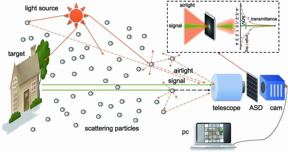
Figure 1.Schematic illustration of the proposed passive imaging through scattering media. ASD, angle-selection device. The inset at the upper-right corner shows that the use of ASD can significantly filter out the light with large incident angles.
B. Improving SIR by ASD
As mentioned above, each component of the signal light arrives at the imaging system with a fixed angle, and most of them come with small ones. In contrast, the arriving angles of the airlight usually obey a more uniform distribution [39]. Based on this characteristic, we propose to improve the SIR of the captured hazy image by blocking the larger-angle components with the use of ASD. As schematically shown in the inset of Fig. 1, ASD accepts incident light with an angle smaller than a critical value and partially rejects those with larger ones.
There are many devices one can employ for this purpose, ranging from conventional gratings to metasurfaces. The ASD we used here was a liquid crystal device that allows an incoming light beam with a small incident angle to transmit. The panel of the liquid crystal is sandwiched between a set of two orthogonally aligned linear polarizers, allowing it to select the polarization state of the incident light as well. This is in particular useful for our application as the airlight usually experiences multiple scattering, and is therefore depolarized.
C. Reducing Airlight Noise by TDMF
We propose to further reduce the noise by taking the temporal fluctuation of the airlight into account. For coherent illumination, each realization of the airlight pattern of a short exposure looks quite random [38] but obeys the same statistics. Thus, one can take advantage of the ergodic property of the process and smooth out the noise by averaging out multiple exposures [38]. However, this strategy does not work well in the case of incoherent illumination in our study because the averaging process has been conducted by the incoherence nature alone [23].
However, we notice that the use of ASD can improve this situation. Although not quite obviously, the airlight pattern acquired through a short exposure with the presence of ASD does have a fluctuation slightly different one from another. This gives us the intuition to develop a spatial filtering algorithm termed as time-domain minimum filtering (TDMF) as shown in Fig. 2. In contrast to the conventional averaging process [38], the proposed TDMF performs noise reduction by
![]()
Figure 2.Schematic illustration of the pipeline of the proposed time-domain minimum filtering (TDMF) algorithm. To enhance image quality through multiple measurements, the proposed TDMF algorithm selects minimal pixel values from multiple frames. Note that CLAHE and DCT are used to further enhance the image contrast.
The justification to pick out the lowest value from , relies on the fact that the ballistic light is too low so that it occupies the lower bit-levels of the camera. In contrast, the airlight is high and occupies the upper bit-levels. The selection of the lowest value from for each pixel means to select the one that has the lowest airlight level.
D. Contrast Enhancement by CLAHE and DCT
After the above two procedures, the signal levels are still lower than those of the airlight. To proceed, we used two standard algorithms, i.e., CLAHE and DCT, to further enhance the contrast. CLAHE is a local histogram equalization algorithm. It divides the image to be processed into a number of small regions called tiles, and performs histogram equalization of them separately. The neighboring tiles are then combined using bilinear interpolation to remove the artificial boundaries.
The pseudocode of the above processing pipeline is shown in Algorithm 1.
| 1: |
| |
| 2: |
| 3: |
| 4: |
| |
| 5: |
| 6: |
| 7: |
| 8: |
| 9: |
| 10: |
| 11: |
| 12: |
| 13: |
Table 1. Pseudocode of the Proposed Algorithm
3. EXPERIMENTAL RESULTS
A. Experimental Setup
Figure 3 depicts the experimental setup and the site map where we performed our outfield experiments. The object to be imaged is two houses shown in Fig. 3(a). The imaging optic shown in Fig. 3(b) was a reflector telescope (CPC1100HD, Celestron) with a 0.27° angle of view (AOV). The ASD (KURIOS-WL1/M, Thorlabs) was placed between the telescope and the camera (PCO Edge4.2). The exact position of it does not have to be precisely specific. The transmittance of ASD is highly angle dependent. It drops quickly when the incident angle of the incoming light changes from 0° to about 6°, as shown in the inset of Fig. 1.
![]()
Figure 3.Sitemap where our outfield experiments were performed. (a) Scene to be imaged and (b) imaging system. The geometric distance between the target and the imager is about 5.9 km.
The experiment was conducted outfield so as to test the performance in a natural environment. The geometric imaging distance is about 5.9 km. However, the presence of the fog changes the optical thickness and therefore the visibility. Since the fog is naturally inhomogeneous along the imaging pathway, we need to measure the equivalent visibility for quantitative analysis.
B. Measurement of the Equivalent Visibility
When light passes through the atmosphere, it obeys the Beer–Lambert law
The optical thickness () is then defined upon this as [22]
The direct measurement of the visibility or the optical thickness over a long distance through an inhomogeneous and thick cloud of fog is extremely challenging. In order to make an approximate estimation of the scattering strength of the fog on site, we controlled an unmanned aerial vehicle (UAV) mounted with a visibility meter to fly all the way from the imaging system to the object, and hover at six different positions at which 10 measurements of the visibility values were taken. Then we determined the local visibility , where , of each of these six positions by averaging out the 10 measured values. In this way, the equivalent visibility of the imaging environment is given by
The experimental result is plotted in Fig. 4; the shadow along the solid line denotes the standard deviation of the measurements. One can see clearly that the equivalent visibility varied from about 1500 m to more than 2400 m during the process when our experiments were carried out.
![]()
Figure 4.Measurement of the equivalent visibility
C. Effectiveness of ASD
The outfield experimental results are shown in Fig. 5. During the course of experiments, the range of visibility of the fog was changing with time, as shown in Fig. 4. One can see from the photo on the left that the scene within this visibility range (450 m) is clear, and the contrast reduces as it goes further (1000 m). Eventually, the signal of the scene is completely immersed in the airlight as its distance (5900 m) is far beyond the range of visibility. This is clearly seen in Figs. 5(a)–5(c), which are the photos of the object 5900 m away in the fog with the equivalent visibility of 2789 m, 2789 m, and 2428 m, respectively. Figure 5(b) is darker than Fig. 5(a) because ASD was used and blocked more light. According to Eq. (2), even in this case, there is still a small amount of signal that can be detected if the camera has enough dynamic range. Thus one can use an image enhancement algorithm, such as the global histogram equalization [42], to enhance the image. The enhanced versions of these three images are shown in Figs. 5(d), 5(e), and 5(f), respectively. One can clearly see by comparing Fig. 5(e) with Fig. 5(d) that the use of ASD indeed helps improve the SIR of the image, even at lower visibility as shown in Fig. 5(f).
![]()
Figure 5.Experimental demonstration of the effectiveness of ASD: single-shot results. The photo on the left (taken by a cell phone) gives an impression of the visibility of the scene. Raw images taken by the PCO camera at the calibrated effective visibility equal to (a) 2789 m without the use of ASD, (b) 2789 m with the use of ASD, (c) 2428 m with the use of ASD, and (d)–(f) SIR enhanced versions of them, respectively, using the global histogram equalization algorithm.
D. Effectiveness of the Proposed Algorithm
When the optical thickness of the fog increases, the visibility range decreases. In another outfield experiment, we took the images [Fig. 6(a)] of the same scene but the equivalent visibility was 2100 m, 1930 m, 1830 m, 1750 m, and 1500 m, respectively. Again, the images look dark because of the use of ASD. The enhanced images by using the proposed algorithm (Fig. 2) are plotted in Fig. 6(c). One can see that the enhanced image is clear and full of detailed structures even when . A traditional algorithm such as the global histogram equalization is also used for image enhancement. The results are shown in Fig. 6(b). One can see that the global histogram equalization algorithm has a worse performance than ours as it reveals fewer structural details of the scene (in particular the windows of the houses) when . As goes down to 1830 m, the windows of the houses become indistinguishable. When the fog grows stronger (), the conventional averaging and global enhancement algorithms fail to reveal many structural details of the scene compared with ours.
![]()
Figure 6.Experimental demonstration of the proposed method, i.e., ASD
4. CONCLUSIONS
In conclusion, we have presented a universal and passive incoherent imaging method for imaging through optically thick scattering media. The proposed method does not rely on any prior of the scene but the co-design of the hardware (i.e., the optical system) and software (i.e., the image enhancement algorithm). This is implemented by the use of ASD to block the large-angle components of the airlight and an algorithm to reconstruct the image from the recorded scattered pattern. But the use of ASD plays a more crucial role.
In outfield experiments, we have demonstrated the performance of the proposed method for imaging a scene with the imaging distance of about 5.9 km through a cloud of fog with different visibility ranges. We believe that the use of more advanced algorithms such as deep learning can further improve the performance.
As we stated in the text, our treatment of the image formation model [Eq. (3)] is based on the assumptions that the fog is stable in density and homogeneous at least within the field of view. It is invalid when these conditions are not satisfied. In addition, as the optical thickness of the fog increases, the attenuation parameter becomes so small that the signal light can be extremely weak, and eventually extinguished completely. This should be the fundamental limit of the proposed method.
References
[4] S. Demos, R. Alfano. Optical polarization imaging. Appl. Opt., 36, 150-155(1997).
[6] D. Huang, E. A. Swanson, C. P. Lin. Optical coherence tomography. Science, 254, 1178-1181(1991).
[8] W. H. Jiang. Adaptive optical technology. Chin. J. Nature, 28, 7-13(2006).
[9] R. H. Webb. Confocal optical microscopy. Rep. Prog. Phys., 59, 427-471(1996).
[12] F. Helmchen, W. Denk. Deep tissue two-photon microscopy. Nat. Methods, 2, 932-940(2005).
[24] E. J. McCartney. Optics of the Atmosphere: Scattering by Molecules and Particles(1976).
[27] Y. Y. Schechner, S. G. Narasimhan, S. K. Nayar. Instant dehazing of images using polarization. IEEE Computer Society Conference on Computer Vision and Pattern Recognition (CVPR), 1, I-I(2001).
[32] W. Ren, L. Ma, J. Zhang. Gated fusion network for single image dehazing. IEEE Conference on Computer Vision and Pattern Recognition, 3253-3261(2018).
[33] P. S. Heckbert, K. Zuiderveld. Contrast limited adaptive histogram equalization. Graphics Gems, 474-485(1994).
[34] S. A. Khayam. The discrete cosine transform (DCT): theory and application. Michigan State Univ., 114, 1-31(2003).
[35] S. K. Nayar, S. G. Narasimhan. Vision in bad weather. 7th IEEE International Conference on Computer Vision, 2, 820-827(1999).
[36] R. T. Tan. Visibility in bad weather from a single image. IEEE Conference on Computer Vision and Pattern Recognition, 1-8(2008).
[37] R. Fattal. Single image dehazing. ACM Trans. Graph., 27, 1-9(2008).
[38] M. J. Beran, J. Oz-Vogt. Imaging through turbulence in the atmosphere. Progress in Optics, 33, 319-388(1994).
[39] A. A. Kokhanovsky. Cloud Optics(2006).
[40] H. Koschmieder. Theorie der horizontalen sichtweite. Beitraege Phys. Atmosp., 12, 33-35(1924).
[41] W. M.. Guide to Meteorological Instruments and Methods of Observation(1996).

Set citation alerts for the article
Please enter your email address
© Copyright 2018-2021 | Chinese Laser Press. All Rights Reserved 沪ICP备15018463号-20