Controlling nonadiabatic spectral redshift of high-order harmonic using two orthogonally polarized laser fields

Hongmei Wu; Shengjun Yue; Jinbin Li; Silin Fu; Bitao Hu; Hongchuan Du

doi:10.3788/COL201816.040203

Abstract

We investigate the nonadiabatic spectral redshift of high-order harmonic of

He

driven by two time-delayed orthogonally polarized laser fields. It is found that the nonadiabatic spectral redshift can be observed by properly adjusting the time delay of the two laser fields when the controlling pulse is added in the raising part of the driving pulse in the vertical direction. That is because the controlling pulse in the vertical direction prevents the ionized electrons from returning to the vicinity of parent ions and then reduces the recombination probability. This leads to the high-order harmonic generated mainly in the falling part of the driving pulse. Meanwhile, we also find that the quantity of redshift can be effectively controlled through accommodating the positive time delays. In addition, this scheme can also be used to produce nonadiabatic spectral blueshift.

High-order harmonic generation (HHG) is one of the most important phenomena in the interaction of atoms or molecules and intense laser fields^[1–3]. The physical mechanism of the HHG can be well described through the semiclassical “three-step model”^[4]. Firstly, the electron tunnels to the continuum state when the Coulomb potential is suppressed by the laser field. Secondly, the ionized electron is accelerated under the driving of the intense laser field, then it reverses the direction of its motion after the laser field changes its sign. Finally, the electron returns to the remaining core and recombines with it to emit a photon. HHG has been a popular topic in both theoretical and experimental studies, since it is a powerful tool to generate isolated attosecond pulses^[5,6] and to probe the electronic and nuclear motion with the temporal resolution on the attosecond time scale^[7].

As a promising method to investigate the ultrafast dynamics of atoms and molecules, the nonadiabatic spectral redshift of high-order harmonic has been studied extensively^[8–11]. For example, Bian et al. found that the harmonic nonadiabatic redshift can be used to extract the internuclear separation^[8]. Besides, the spectral redshift can be used to produce the adjustable frequency combs in the ultraviolet or extreme ultraviolet spectral region. The nonadiabatic spectral shift comes from the broken balance between the blueshift in the raising part of the laser pulse and the redshift in the falling part of the laser pulse (Ref. [8] for details). Once the contribution of the falling part of the laser pulse to high-order harmonics is predominant, the nonadiabatic spectral redshift would be observed. So far, there have been many efforts to produce the nonadiabatic spectral redshift. As Bian et al.^[12] studied earlier, the nonadiabatic spectral redshift can be produced from the asymmetric diatomic molecule ${HeH}^{2 +}$ with long-life excited state in a short intense laser pulse, since the long lifetime of the excited state leads to the enhanced ionization in the falling part of the laser pulse. Subsequently, they investigated the orientation^[13] and pulse duration dependence^[8] of nonadiabatic spectral redshift in molecular HHG (MHOHG). Unfortunately, the appearance of the nonadiabatic spectral redshift of atoms and ions is not involved. In view of this point, we have recently studied the nonadiabatic spectral redshift of ${He}^{+}$ by adding a 13th harmonic pulse^[14,15] to the falling part of the fundamental laser pulse. However, as shown above, the nonadiabatic spectral redshift is mainly produced by controlling the ionization process so far. To the best of our knowledge, the generation of the nonadiabatic spectral redshift is hardly reported by controlling the recombination process. Therefore, in this work, we investigate the nonadiabatic spectral redshift of He by controlling the recombination process. In order to control the recombination process effectively, a controlling pulse is added in the raising part of the driving pulse in the vertical direction, which is shown in Fig. 1. By means of this scheme, the nonadiabatic spectral redshift can be obtained by adjusting the time delay between the two laser pulses. Moreover, this scheme can also produce the nonadiabatic spectral blueshift. Finally, it is found that the quantity of redshift can be effectively controlled through accommodating the positive time delays. Compared with the method by controlling the ionization rate, adjusting the time delay of the two orthogonally polarized laser fields is more practical in experiment.

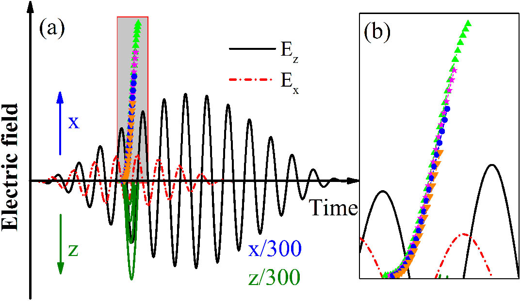
Figure 1.(a) Two orthogonally polarized laser electric fields and trajectories of ionized electrons in the laser pulses. The black curve is the driving field polarized along the $z$ axis, and the red short dash dot curve is the controlling field polarized along the $x$ axis. The olive curves and the colorful line with symbol curves represent the electrons’ trajectories regulated by the driving field and the controlling field, respectively. For clarity, the trajectories are reduced by 300 times. (b) The enlargement of the shadow area in (a).

In order to investigate the interaction between $He$ and the two orthogonally polarized laser fields, we numerically solve the three-dimensional (3D) time dependent schrödinger equation (TDSE) with the single-active-electron (SAE) approximation^[16] in the length gauge. The TDSE in the cylindrical coordinate system^[17] can be described as (atomic units are used throughout unless stated otherwise) $i \frac{\partial}{\partial t} ψ (ρ, z, ϕ; t) = \hat{H} ψ (ρ, z, ϕ; t) .$ (1)

Sign up for Chinese Optics Letters TOC. Get the latest issue of Chinese Optics Letters delivered right to you！Sign up now

The Hamiltonian is given by $\hat{H} = - \frac{1}{2} (\frac{\partial^{2}}{\partial ρ^{2}} + \frac{1}{ρ} \frac{\partial}{\partial ρ} + \frac{\partial^{2}}{\partial z^{2}} + \frac{1}{ρ^{2}} \frac{\partial^{2}}{\partial ϕ^{2}}) + V (ρ, z) - \vec{z} \cdot \vec{E} (t) - \vec{x} \cdot \vec{E} (t),$ (2)where $V (ρ, z) = - \sqrt{2 I_{p}} / \sqrt{ρ^{2} + z^{2}}$ is the effective potential, and $I_{p}$ is the ionization energy of $He$ . The TDSE is solved by using the Crank–Nicolson method^[18]. After the wave function is obtained, the time-dependent dipole acceleration can be expressed as $\vec{a} (t) = - 〈 ψ (\vec{r}, t) | \nabla [V (\vec{r}) + \vec{r} \cdot \vec{E} (t)] | ψ (\vec{r}, t) 〉,$ (3)where $\vec{r} = (ρ, z, ϕ)$ denotes the position of the electron. Finally, one can gain the high-order harmonic spectrum through the Fourier transform of the dipole acceleration: $F (ω) = {| \frac{1}{2 π} \int_{- \infty}^{+ \infty} \vec{a} (t) e^{- i ω t} d t |}^{2} .$ (4)

The electric field $\vec{E} (t)$ used in the calculation is defined as $\vec{E} (t) = {\vec{E}}_{z} (t) + {\vec{E}}_{x} (t) = E_{z 0} \sin^{2} (\frac{π t}{τ_{1}}) \sin (ω t) \cdot {\vec{e}}_{z} + E_{x 0} \sin^{2} [\frac{π (t + t_{delay})}{τ_{2}}] \sin [ω (t + t_{delay})] \cdot {\vec{e}}_{x} .$ (5)

In this equation, ${\vec{E}}_{z}$ is the driving pulse, ${\vec{E}}_{x}$ is the controlling pulse, and $E_{z 0}$ and $E_{x 0}$ are the electric peak amplitudes of the two orthogonally polarized laser pulses, respectively. $ω$ is the angular frequency. $τ_{1}$ and $τ_{2}$ are the duration of ${\vec{E}}_{z}$ and ${\vec{E}}_{x}$ , respectively. $t_{delay}$ is defined as the time delay. The symbols ${\vec{E}}_{z}$ and ${\vec{e}}_{x}$ denote the unit vector along the $z$ and $x$ axes, respectively. The grids are set as $0 a.u. < ρ < 60 a.u.$ , $- 60 a.u. < z < 60 a.u.$ with the spatial step $d ρ = d z = 0.1 a.u.$ , and the propagating time step is $d t = 0.05 a.u.$ . Adopting $\frac{1}{2} d ρ$ as the initial value of $ρ$ and considering the cylindrical coordinate symmetry of the wave function, one can overcome the singularity of the potential V in the TDSE simulations. To prevent non-physical reflection at the boundary, we apply the absorbing function $f_{a p} = \cos {[\frac{π (| ρ | - ρ_{0})}{ρ_{\max} - ρ_{0}}]}^{1 / 8}$ when $ρ_{0} < | ρ | < 60 a.u.$ , and $f_{z p} = \cos {[\frac{π (| z | - z_{0})}{z_{\max} - z_{0}}]}^{1 / 8}$ when $z_{0} < | z | < 60 a.u.$ ; $ρ_{0}$ and $z_{0}$ are the initial positions of the absorbing function. In order to suppress the interference between the long trajectories and the short trajectories^[7,19], $ρ_{0}$ and $z_{0}$ are set as $0.9 E_{x 0} / ω^{2}$ and $0.9 E_{z 0} / ω^{2}$ , respectively, thereby wiping out the long trajectories^[20,21]. In experiment, the long trajectories can be eliminated by putting the gas jet after the laser focus^[22–24].

In our scheme, the driving pulse and the controlling pulse are adopted to manipulate the ionization and recombination processes, respectively. As shown in Fig. 1(a), when the controlling pulse is added in the raising part of the driving pulse with $t_{delay} = 0.25 T$ , the driving pulse will regulate the trajectories of ionized electrons along the $z$ axis (olive solid curves), and the controlling pulse will regulate the trajectories along the $x$ axis (colorful line with symbol curves). Figure 1(b) shows the enlarged trajectories along $x$ . Because the driving and controlling pulses do not change their sign simultaneously, there is a disparity between the returning time of the ionized electron in the two directions. Therefore, the electron cannot return to the parent ion in the $x$ direction, as shown in Fig. 1(b), when it returns to the parent ion in the $z$ direction. Hence, the contribution of the raising part to the harmonic is smaller than that of the falling part, resulting in the nonadiabatic spectral redshift of high-order harmonics.

In order to demonstrate this scheme, the high-order harmonic spectra of the $He$ atom exposed to the driving pulse and the combined field are presented in Figs. 2(a) and 2(b), respectively. In the combined eld whose wavelength is 800 nm, the controlling pulse is added in the rising part of the driving pulse. In our calculation, two orthogonally polarized laser pulses with an 800 nm wavelength are adopted, and the durations of the driving and the controlling pulses are set as $15 T$ ( $T$ is the optical cycle period) and $10 T$ , respectively. $t_{delay}$ is equal to $0.25 T$ . The electric peak amplitudes of the driving and controlling pulses are chosen as 0.1 and 0.03 a.u., respectively. The structures of the harmonic spectra in Fig. 2 are very similar to each other. While by comparing the harmonic spectra in the top right corners of Figs. 2(a) and 2(b), one can note that there are only odd harmonics in Fig. 2(a), but distinct spectral redshift in Fig. 2(b).

Figure 2.(a) High-order harmonic spectra of $He$ in the driving pulse. (b) High-order harmonic spectra of He in two orthogonally polarized laser pulses. The top right corners of (a) and (b) are the partially enlarged details.

In order to gain insight into the mechanism of the red shift, the time-frequency analyses of the harmonic spectra are shown in Fig. 3. Because the low-order harmonics are more complicated, we only focus on the plateau region of the harmonic spectra. For harmonics generated in the driving pulse, as shown in Fig. 3(a), the contributions of the raising part and the falling part to high-order harmonics are almost identical. Hence, there is no net redshift observed in Fig. 2(a). However, for the harmonics generated in the combined pulse, the contribution of the raising part to high-order harmonics is lower than that in the falling part. Hence, the balance of the HHG is broken, and the redshift can be observed, as shown in Fig. 2(b). Moreover, to clearly understand the relation between the redshift and the broken symmetry, we further calculate the asymmetry coefficients^[11] of high-order harmonics in the plateau region by $A (ω_{N}) = \frac{P_{R} (ω_{N}) - P_{L} (ω_{N})}{P_{R} (ω_{N}) + P_{L} (ω_{N})},$ (6)where $P_{L} (ω_{N}) = \int_{0}^{τ_{1} / 2} g (ω_{N}, t) d t$ , $P_{R} (ω_{N}) = \int_{τ_{1} / 2}^{τ_{1}} g (ω_{N}, t) d t$ , $P_{L} (ω_{N})$ , and $P_{R} (ω_{N})$ are defined as the total harmonic $ω_{N}$ generated in the raising part and the falling part of the driving pulse, respectively. $g (ω_{N})$ is the time-frequency intensity of the $N$ th harmonic at time $t$ . The results are shown in Fig. 4(b), which indicate that the contribution of the falling part of the laser pulse to the high-order harmonics is larger than that of the raising part. Figure 4(a) presents the quantity of the redshift. The overall trend is on the rise, which accords with the asymmetry coefficients qualitatively.

Figure 3.Time-frequency analysis of harmonic spectra (a) in the driving pulse and (b) in the two orthogonally polarized laser pulses.

Figure 4.Spectral redshift of high-order harmonics and asymmetry coefficients.

As above shown, the redshift comes from the broken balance of the blueshift in the raising part and the redshift in the falling part, in which the redshift predominates. However, what brings about the breach of the balance in our scheme, the ionization process or recombination process? To solve this problem, we calculate the ionization rate of $He$ in the driving laser pulse and in the two orthogonally polarized laser pulses, respectively. Just as presented in Fig. 5, the ionization rate of $He$ in the driving pulse and in the two laser pulses are almost same. Thus, we can conclude that the recombination process breaches the balance. Besides, the collective response of the macroscopic gas has an important effect on the harmonic spectra^[25,26], and the ionization rate of the gas target determines the collective response^[27] when the focusing geometry of the laser pulse remains unchanged. Therefore, the impact of the collective response on the harmonic spectra is identical for these two cases. Hence, one can offset the effect of the collective response on the harmonic spectra by comparing the harmonic spectrum in the combined laser pulses with that in the driving pulse and further obtain the value of the nonadiabatic spectral redshift.

Figure 5.Ionization rate of $He$ at different times. The red solid curve represents the ionization rate in the driving pulse, and the blue short dash curve represents the ionization rate in the two orthogonally polarized laser pulses.

When the controlling pulse is added to the falling part of the driving pulse with a proper time delay, $t_{delay} = 4.75 T$ for instance, the nonadiabatic spectral blueshift will be produced. In order to confirm it, we calculate the harmonic spectrum and perform the corresponding time-frequency analysis with $t_{delay} = 4.75 T$ . The results are presented in Figs. 6(a) and 6(b), respectively. From Fig. 6(a), one can observe an obvious blueshift. Further time-frequency analysis, shown in Fig. 6(b) confirms that the contributions of the raising part of the driving pulse to the high-order harmonics is larger than that of the falling part as expected.

Figure 6.(a) The harmonic spectrum and (b) the corresponding time-frequency analysis. The controlling pulse is added in the falling part of the driving pulse with $t_{delay} = 4.75 T$ . The top right corner of (a) is the partially enlarged details.

Finally, we discuss the effect of positive and negative time delays^[28] on the harmonic redshift when the controlling pulse is added in the raising part of the driving pulse. In this section, four pairs of harmonic spectra calculated with positive and negative time delays are shown in Figs. 7(a) and 7(b), respectively. In Fig. 7(a), it is clear that the redshift becomes larger with the increasing positive time delays, meanwhile the intensity tends to decrease gradually. Besides, the redshift in the laser fields with negative time delays has a similar trend for some harmonics, but the trend is not obvious, as shown in Fig. 7(b).

Figure 7.Partial harmonic spectra for different time delays between the two orthogonally polarized laser fields with (a) positive time delays and (b) negative time delays. The orange dash lines correspond exactly to odd harmonics.

In order to further understand the effect of positive and negative time delays on the harmonic generation, the “three-step” model^[4] is applied in our calculation. One can see from Fig. 8(a) that the tunneling electron contributing to the 33th harmonic ionizes at $5.82 T$ and recombines at $6.28 T$ under the control of the driving pulse. As shown in Fig. 8(b), the distance of the electrons to the nuclei becomes farther with the increasing positive time delays. This leads to the decrease of the recombination rate in the raising part of the laser field, which exacerbates the imbalance of the redshift and the blueshift. That is why the redshift is more and more obvious, as presented in Fig. 7(a). For electrons in the two laser fields with negative time delays, the distance between the electrons and the nuclei at the recombination moment in the $z$ direction also goes up with the increasing time delays, as depicted in Fig. 8(c). However, the change of the redshift in Fig. 7(b) is not obvious. The distinction of the redshift trend can be explained by the electric fields of the two laser pulses. When the time delay is positive, the peak field of the controlling pulse is left compared with that of the driving pulse, while it shifts to the right for the negative time delays. In this case, since the peak field of the driving pulse is followed by that of the controlling pulse, the ionized electron near the peak of the driving pulse runs away from the parent ion directly when it returns to the parent ion in the $z$ direction. Therefore, the change of the redshift for different time delays is not obvious. So, it is better to control the nonadiabatic spectral redshift by adjusting the positive time delays.

Figure 8.(a) Harmonic orders of different recombination moments, and the relation between the ionization moment (red circle) and recombination moment (violet short dash curve) in the $z$ direction for electrons ionized from $5.75 T$ to $6.0 T$ . The black solid curve represents the partial driving field. The olive and orange triangles point to the ionization time and recombination time of the 33th harmonic, respectively. (b) and (c) demonstrate trajectories of electrons along the $x$ direction in the two laser fields with positive and negative time delays, respectively. The starting and ending times correspond to triangle marks in (a).

In conclusion, we theoretically investigated the redshift of high-order harmonics of $He$ by numerically solving 3D TDSE in a length gauge. In our work, by adding a controlling field to the raising part of the driving field with a proper time delay, the nonadiabatic spectral redshift of high-order harmonics can be produced. Since the ionization rates in the driving field and in the combined laser fields are almost the same, we confirm that the nonadiabatic spectral redshift results from the recombination process. Moreover, this scheme can also be used to produce a nonadiabatic spectral blueshift of high-order harmonics by adding the controlling field to the falling part of the driving field. At the end of the Letter, the effect of positive and negative time delays on the nonadiabatic spectral redshift is also studied. It is found that the quantity of redshift can be effectively controlled by adjusting the positive time delays. The laser parameters used in the current work are currently, experimentally accessible. It is hoped that this scheme will be achieved in experiments.

References

[1] J. L. Krause, K. J. Schafer, K. C. Kulander. Phys. Rev. Lett., 68, 3535(1992).

[2] J. Zhang, X. Ge, T. Wang, T. Xu, J. Guo, X. Liu. Phys. Rev. A, 92, 013418(2015).

[3] X. L. Yuan, C. D. Liu, P. F. Wei, Z. N. Zeng, R. X. Li. Chin. Opt. Lett., 14, 030201(2016).

[4] P. B. Corkum. Phys. Rev. Lett., 71, 1994(1993).

[5] C. Yu, H. He, Y. Wang, Q. Shi, Y. Zhang, R. Lu. J. Phys. B: At. Mol. Opt. Phys., 47, 055601(2014).

[6] L. Li, C. Xia, X. Miao. Spectrosc. Lett., 49, 231(2016).

[7] P. Lan, M. Ruhmann, L. He, C. Zhai, F. Wang, X. Zhu, Q. Zhang, Y. Zhou, M. Li, M. Lein, P. Lu. Phys. Rev. Lett., 119, 033201(2017).

[8] X. Bian, A. D. Bandrauk. Phys. Rev. Lett., 113, 193901(2014).

[9] Y. H. Gu, C. Z. Cai, Q. Feng, Y. H. Li. Chin. Opt. Lett., 12, 091602(2014).

[10] H. Ahmadi, M. Vafaee, A. Maghari. Phys. Rev. A, 94, 033415(2016).

[11] M. Li, G. Jia, X. Bian. J. Chem. Phys., 146, 084305(2017).