Performance analysis of ghost imaging lidar in background light environment

Chenjin Deng; Long Pan; Chenglong Wang; Xin Gao; Wenlin Gong; Shensheng Han

doi:10.1364/PRJ.5.000431

Abstract

The effect of background light on the imaging quality of three typical ghost imaging (GI) lidar systems (namely narrow pulsed GI lidar, heterodyne GI lidar, and pulse-compression GI lidar via coherent detection) is investigated. By computing the signal-to-noise ratio (SNR) of fluctuation-correlation GI, our analytical results, which are backed up by numerical simulations, demonstrate that pulse-compression GI lidar via coherent detection has the strongest capacity against background light, whereas the reconstruction quality of narrow pulsed GI lidar is the most vulnerable to background light. The relationship between the peak SNR of the reconstruction image and σ (namely, the signal power to background power ratio) for the three GI lidar systems is also presented, and the results accord with the curve of SNR-σ.

Keywords

(110.1758) Computational imaging.(110.2990) Image formation theory (110.0110) Imaging systems

1. INTRODUCTION

Ghost imaging (GI) is a novel non-scanning imaging method to obtain a target’s image with a single-pixel bucket detector ^[1–6]. Due to its capacity for high detection sensitivity, GI has aroused increasing interest in remote sensing, and a new imaging lidar system called GI lidar has gradually developed ^[7–15]. Up to now, there have been three types of three-dimensional GI lidars, namely narrow pulsed GI lidar, heterodyne GI lidar, and pulse-compression GI lidar via coherent detection ^[12–15]. Due to their distinct mechanisms, their advantages and disadvantages are obviously different. For narrow pulsed GI lidar, a series of high-power laser pulses with independent speckle configurations illuminate onto the target, and the backscattered intensity is directly received by a time-resolved bucket detector ^[7–13]. The structure of pulsed GI lidar is simple, but its imaging quality is subject to a low-detection signal-to-noise ratio (SNR). Heterodyne GI lidar employs a spatiotemporal modulated light generated by temporal chirped amplitude modulation (chirped-AM) and transverse random modulation ^[14]. Using a de-chirping method, a high-range resolution can be obtained even with the use of a long pulse. However, similar to narrow pulsed GI lidar, heterodyne GI lidar uses a direct light-detection mechanism, which leads to a shorter detection distance because the laser’s power is relatively low compared with narrow pulsed GI lidar. Pulse-compression GI lidar via coherent detection shares similar spatiotemporal light with heterodyne GI lidar, but its detection mechanism is based on coherent detection ^[15]. Pulse compression gives this lidar high-range resolution, long detection range, and insensitivity to stray light. However, in order to ensure heterodyne efficiency, the laser’s line width is usually very narrow and the numerical aperture of the receiving system should be very small. In remote-sensing GI lidar detection applications, background light is inevitable and its intensity may be greater than the intensity of the signal. Therefore, it would be very useful to clarify the influence of background light on the imaging quality of GI lidar systems.

In this paper, the performance of the three aforementioned GI lidar systems is analyzed in a background light environment. In Section 2, we theoretically analyze the imaging SNR of pulsed GI lidar, heterodyne GI lidar, and pulse-compression GI lidar via coherent detection, when the signal light is contaminated by background light. Following the analysis, we give a numerical simulation to demonstrate the performance of these systems under different levels of background light in Section 3. Finally, a conclusion is made in Section 4.

2. SYSTEM ANALYSIS

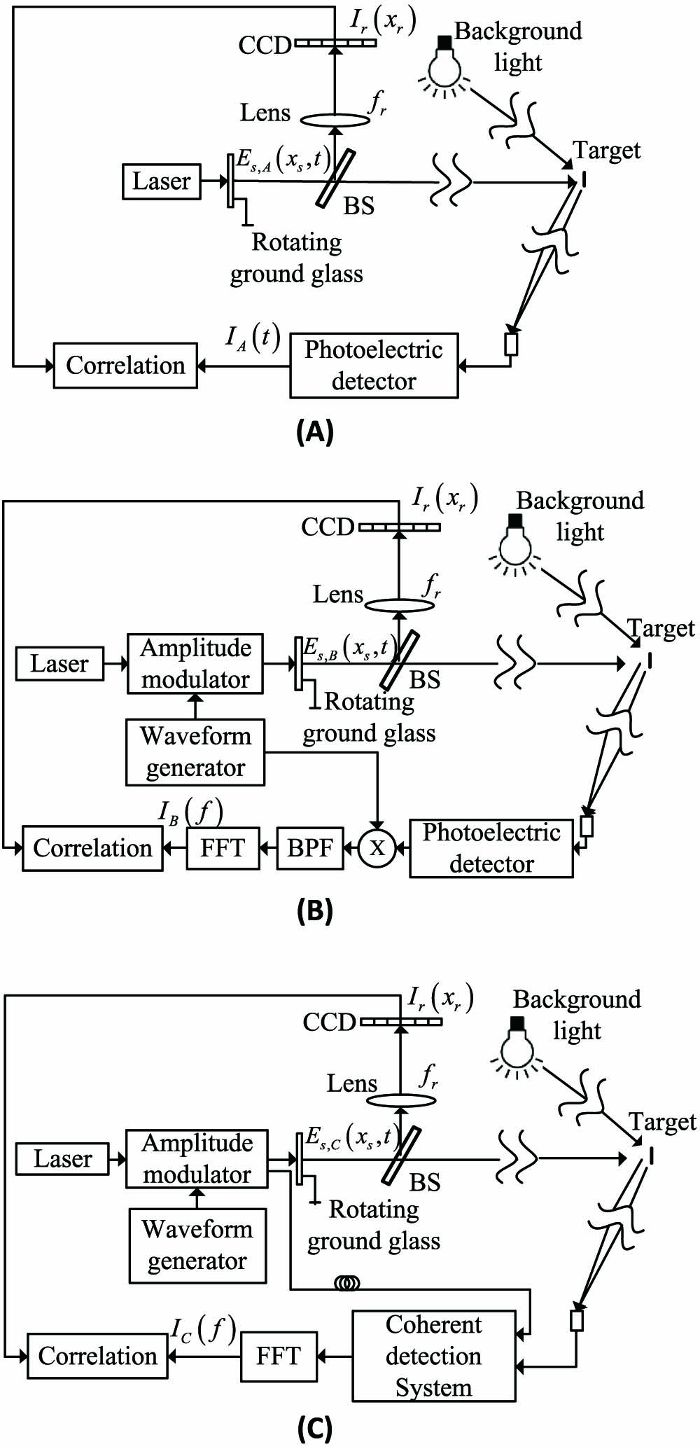
Figure 1 is the schematic of the three different types of GI lidar: (A) narrow pulsed GI lidar, (B) heterodyne GI lidar, and (C) pulse-compression GI lidar via coherent detection. In these lidar systems, modulated light pulses are generated and divided into reference and test paths by a beam splitter (BS). In the reference path, the light’s far-field intensity distribution $I (x_{r})$ is recorded by a CCD camera, where $x_{r}$ is the coordinate on the CCD plane. In the test path, light propagates to the target and the backscattered light field propagates to the receiving aperture. Through different kinds of receiving methods, the light intensity $I_{i}$ is obtained, where $i = A, B, C$ . Performing the spatial correlations between the output signal $I_{i}$ and $I_{r} (x_{r})$ respectively, we try to reconstruct the image, namely where $⟨ ⟩$ is an average over independent speckle configurations, $δ I_{i} = I_{i} - ⟨ I_{i} ⟩$ , and $δ I_{i} (x_{r}) = I_{i} (x_{r}) - ⟨ I_{i} (x_{r}) ⟩$ . The noise associated with $G_{i} (x_{r})$ is ^[4,5]

Sign up for Photonics Research TOC. Get the latest issue of Photonics Research delivered right to you！Sign up now

Schematic of GI lidar via different detection mechanisms: (A) narrow pulsed GI lidar, (B) heterodyne GI lidar, and (C) pulse-compression GI lidar via coherent detection.

Figure 1.Schematic of GI lidar via different detection mechanisms: (A) narrow pulsed GI lidar, (B) heterodyne GI lidar, and (C) pulse-compression GI lidar via coherent detection.

Following Refs. ^[16,17], we define the minimum variation of $Δ ⟨ G_{i} ⟩$ as the signal that needs to be detected, and thus the image SNR for lidar systems (A)–(C) is

In these three lidar systems, a modulated light pulse can be denoted as where $x_{s}$ is the coordinate on the source plane, $s_{i} (t)$ is a temporal modulation, and $E_{s} (x_{s})$ is the spatial modulation. For lidar system (A), $s_{A} (t) = Rect (t / T_{A})$ , where $Rect (t / T)$ is a rectangular window function and is time limited in $0 < t < T$ . Lidar systems (B) and (C) share a similar modulation system, namely $s_{B} (t) = s_{C} (t) = [1 + m s_{chirp} (t)] Rect (t / T_{chirp})$ , where $s_{chirp} (t)$ is a chirped-AM waveform with bandwidth $B_{chirp}$ and duration $T_{B} = T_{C} = T_{chirp}$ , and $m$ is the modulation depth ^[14,15]. To obtain equivalent range resolution, we set $B_{chirp} = 1 / T_{A}$ .

In practical lidar applications, background light is inevitable, which will reduce the detection SNR. As Fig. 1 shows, background light can be treated as an extra light source illuminating the target. Thus, the total light field on the target plane can be modeled as the sum of signal light and background light, namely where $x_{o}$ is the coordinate on the target plane and $E_{s, i} (x_{o}, t)$ , $E_{b g} (x_{o}, t)$ denotes the signal and background light fields, respectively. In the following analysis, the background light is modeled as a random filed whose amplitude and phase are random functions of coordinate and time, namely $E_{b g} (x_{o}, t) = A_{b g} (x_{o}, t) \exp [j ϕ_{b g} (x_{o}, t)]$ , which satisfies where $⟨ I_{b g} ⟩$ is the average background light power, $K_{b g} (t)$ is the spatial part of the correlation function, and $R_{b g} (t)$ is the temporal part with coherence time $τ_{b g}$ much shorter than both integration time of the photodetector and pulse duration $T_{i}$ ^[18]. The speckle coherence area of the background and signal light fields can be defined as $A_{coh, bg} = \int {| K_{b g} (x) |}^{2} d x$ and $A_{coh, s} = \int {| μ_{s} (x_{o}) |}^{2} d x_{o}$ , where $μ_{s} (x_{o})$ is the mutual complex coherence factor of $E_{s} (x_{o})$ ^[19]. For simplicity, we also assume the three GI systems have uniform illumination (namely average power $⟨ I_{s} (x_{o}) ⟩ = ⟨ I_{s} ⟩$ , $⟨ I_{r} (x_{r}) ⟩ = ⟨ I_{r} ⟩$ ) and perfect resolution. Further, we denote the signal power to background power ratio as $σ (λ) = ⟨ I_{s} (λ) ⟩ / ⟨ I_{b g} (λ) ⟩$ , where $λ$ is the optical wavelength. In the paper, we only consider background light with the same wavelength as the lidar system, since background light of other wavelengths can be filtered out by narrow bandpass filters.

The total light field is reflected by the target, and then received in the detection system. Obviously, the background light will destroy the correlation between the test path and reference path, and thus may affect the quality of the image reconstruction. Since lidar systems (A)–(C) have different detection mechanisms, we will analyze their detection output and image SNR. For simplicity, the conversion factor of the photoelectric detector used in the three lidar systems is assumed to be identical, and thus is ignored in the following analysis.

A. Lidar System (A)

For lidar scheme (A), a time-resolved bucket detector is used to collect the backscattered light. Since the background light’s coherence time $τ_{b g}$ is much shorter than the detector’s integration time, if we ignore the time delay of propagation, the output can be denoted as $I_{A} = \int_{0}^{T_{A}} d t \int_{A_{beam}} d x_{o} [{| E_{s} (x_{o}, t) |}^{2} + {| E_{b g} (x_{o}, t) |}^{2}] O (x_{o}) ≜ I_{A, s} + I_{A, b g},$ (7)where $O (x_{o})$ is the intensity reflection coefficient of the target, and $A_{beam}$ is the area of the light beam. By substituting Eq. (7) into Eq. (1), under a perfect resolution assumption, we can obtain $⟨ G_{A} (x_{r}) ⟩ = T_{A} A_{coh, s} ⟨ I_{r} ⟩ ⟨ I_{s} ⟩ O .$ (8)Since $I_{A, s}$ and $I_{A, b g}$ are independent of each other, by substituting Eq. (7) into Eq. (2), we get $⟨ Δ G_{A}^{2} ⟩ = [⟨ δ I_{A, s}^{2} δ I_{r}^{2} ⟩ - {⟨ δ I_{A, s} δ I_{r} ⟩}^{2}] + ⟨ δ I_{A, b g}^{2} ⟩ ⟨ δ I_{r}^{2} ⟩ = ⟨ δ I_{A, s}^{2} ⟩ ⟨ δ I_{r}^{2} ⟩ + ⟨ δ I_{A, b g}^{2} ⟩ ⟨ δ I_{r}^{2} ⟩ = T_{A}^{2} A_{beam} A_{coh, s} {⟨ I_{r} ⟩}^{2} {⟨ I_{s} ⟩}^{2} \bar{O^{2}} (1 + \frac{τ_{b g}}{T_{A}} \frac{A_{coh, b g}}{A_{coh, s}} \frac{1}{σ^{2}}),$ (9)where $⟨ δ I_{A, s}^{2} δ I_{r}^{2} ⟩ - {⟨ δ I_{A, s} δ I_{r} ⟩}^{2} = ⟨ δ I_{A, s}^{2} ⟩ ⟨ δ I_{r}^{2} ⟩$ is the inherent noise for GI without detection noise ^[16], and $\bar{O^{2}} = \int ⟨ I_{s} ⟩ O^{2} (x_{o}) d x_{o} / \int ⟨ I_{s} ⟩ d x_{o} \approx \int ⟨ I_{s} ⟩ O^{2} (x_{o}) d x_{o} / A_{beam}$ is the average quadratic reflection function of the target. If we average over $N$ independent measurements, using Eqs. (3), (8), and (9), we have ${SNR}_{A} = \frac{N}{N_{sp}} \frac{Δ O_{\min}^{2}}{[1 + \frac{τ_{b g}}{T_{A}} \frac{A_{coh, b g}}{A_{coh, s}} \frac{1}{σ^{2}}] \bar{O^{2}}},$ (10)where $N_{sp} = A_{beam} / A_{coh, s}$ is the number of speckles in the beam and $Δ O_{\min}$ is the minimum variation of the object reflection function to be detected.

B. Lidar System (B)

For lidar system (B), the backscattered light is converted into an intensity-modulated photocurrent $i_{B} (t)$ . Then de-chirping is processed by mixing the photocurrent with a local chirp signal $s_{LO} = s_{chirp}$ . After a proper bandpass filter, fast Fourier transform (FFT) is used to find the beating frequency $f_{z}$ and accumulate the signal energy ^[14]. The amplitude spectrum can be denoted as $I_{B} (f) = FFT {[s_{LO} (t) i_{B} (t)] \otimes H_{B} (t)} = \frac{m}{2} T_{B} sinc [T_{B} (f - f_{z})] \exp [j ϕ_{B}] \int d x_{o} {| E_{B_{s}} (x_{o}, t) |}^{2} O (x_{o}) + FFT {s_{LO} (t) [(\int d x_{o} {| E_{b g} (x_{o}, t) |}^{2} O (x_{o})) \otimes H_{B} (t)]} ≜ I_{B, s} (f) + I_{B, b g} (f),$ (11)where $H_{B} (t)$ is the impulse response function for receiving system (B), $sinc (x) = \sin (π x) / x$ , $ϕ_{B}$ is a constant delay phase, and $\otimes$ denotes convolution. Similar to the process of lidar system (A), by substituting $I_{B} (f_{z})$ into Eqs. (1) and (2), we can obtain the reconstruction image, $⟨ G_{B} (x_{r}) ⟩ = \frac{m}{2} T_{B} A_{coh, s} ⟨ I_{r} ⟩ ⟨ I_{s} ⟩ O,$ (12)and the associated noise, $⟨ Δ G_{B}^{2} ⟩ = \frac{m^{2}}{4} T_{B}^{2} A_{coh, s} A_{beam} {⟨ I_{r} ⟩}^{2} {⟨ I_{s} ⟩}^{2} \bar{O^{2}} \times (1 + \frac{2}{m^{2}} \frac{τ_{b g}}{T_{B}} \frac{A_{coh, b g}}{A_{coh, s}} \frac{1}{σ^{2}}) .$ (13)

Therefore, by substituting Eqs. (12) and (13) into Eq. (3), and averaging over $N$ measurements, we can obtain the image SNR for lidar system (B) as ${SNR}_{B} = \frac{N}{N_{sp}} \frac{Δ O_{\min}^{2}}{[1 + \frac{2}{m^{2}} \frac{τ_{b g}}{T_{B}} \frac{A_{coh, b g}}{A_{coh, s}} \frac{1}{σ^{2}}] \bar{O^{2}}} .$ (14)

C. Lidar System (C)

In lidar system (C), the light signal is mixed with the local chirped-AM modulated light $E_{LO} (t) = [1 + m s_{chirp} (t)] A_{LO} \exp [j ϕ_{LO}]$ , and the range delay signal is converted to a beating frequency $f_{z}$ . Then FFT is applied to find the beating frequency, and a random sparse point detector array is used as an equivalent bucket detector. Finally, the intensity spectrum can be denoted as ^[15] $I_{C} (f_{z}) = \sum_{x_{t}} \frac{m^{4}}{4} T_{C}^{2} I_{LO} I_{s} (x_{t}) + \sum_{x_{t}} {| i_{C, b g} (x_{t}, f_{z}) |}^{2} + 2 Re {\sum_{x_{t}} [m^{2} I_{LO} T_{C} \exp (j ϕ_{C}) E_{s} (x_{t})] {[i_{C, b g} (x_{t}, f_{z})]}^{*}} ≜ I_{C, s} (f_{z}) + I_{C, b g} (f_{z}) + I_{C, m u} (f_{z}),$ (15)where $I_{LO} = {| E_{LO} |}^{2}$ , $ϕ_{C}$ is a constant phase, and $i_{C, b g} (x_{t}, f_{z})$ is the spectrum of background light output. Similar to lidar system (B), the image is retrieved by correlating $I_{C} (f_{z})$ with the reference speckle configurations. By substituting Eq. (15) into Eqs. (1) and (2) respectively, we can obtain $⟨ G_{C} (x_{r}) ⟩ = \frac{m^{4}}{4} I_{LO} T_{C}^{2} A_{coh, s} ⟨ I_{r} ⟩ ⟨ I_{s} ⟩ O$ (16) $⟨ Δ G_{C}^{2} ⟩ = \frac{m^{8}}{16} I_{LO}^{2} T_{C}^{4} A_{beam} A_{coh, s} {⟨ I_{r} ⟩}^{2} {⟨ I_{s} ⟩}^{2} \bar{O^{2}} \times [1 + \frac{64 {(2 + m^{2})}^{2}}{m^{8}} {(\frac{τ_{b g}}{T_{C}})}^{2} \frac{A_{coh, b g}}{A_{coh, s}} \frac{{⟨ I_{b g} ⟩}^{2}}{{⟨ I_{s} ⟩}^{2}}] .$ (17)

Thus, the SNR for lidar system (C) is ${SNR}_{C} = \frac{N}{N_{sp}} \frac{Δ O_{\min}^{2}}{[1 + \frac{64 {(2 + m^{2})}^{2}}{m^{8}} {(\frac{τ_{b g}}{T_{C}})}^{2} \frac{A_{coh, b g}}{A_{coh, s}} \frac{1}{σ^{2}}] \bar{O^{2}}} .$ (18)

As shown by Eqs. (10), (14), and (18), the three lidar systems have different responses to signal and background light, thus leading to different image SNRs when the three systems share the same signal power to background power ratio $σ$ . We will compare them explicitly in the next section.

3. NUMERICAL SIMULATION

In order to demonstrate the performance of these three GI lidar systems under background light, a numerical simulation is performed. The pulse duration for lidar (A) is $T_{A} = 1 ns$ , and the chirped modulation parameters are $T_{chirp} = 400 μs$ and $B_{chirp} = 1 GHz$ ; thus, the range resolutions are identical for the three lidar systems. The specific parameters for transverse modulation are also identical for the three systems, namely $λ = 1550 nm$ , $D_{s} = 2 mm$ , and $f_{r} = 250 mm$ . For simplicity, we only simulate a single static planar target with letters “GI” (the transverse size is about $3 m \times 3 m$ ) at range $z = 200 m$ . The measurement number is $N = 10000$ . A random sparse detector array with 25 point detectors is used for lidar systems (A)–(C).

Figure 2 is the reconstruction images with different levels of average signal power to background power ratio. The signal power to background power ratio $σ$ is $- 40$ , $- 30$ , $- 20$ , $- 10$ , 0, and 10 dB for columns (1)–(6), respectively, and rows (A)–(C) correspond to lidar systems (A)–(C), respectively. As $σ$ becomes weaker, the image quality for every lidar decays. For lidar (A), when $σ \leq 0 dB$ , it fails to reconstruct the image; for lidar (B), the reconstructed image is satisfactory when $σ = - 20 dB$ . Lidar (C) can still reconstruct the image when $σ = - 30 dB$ . Among the three systems, therefore, lidar (C) has the best anti-background-light performance.

Figure 2.Image reconstruction results. The signal power to background power ratio $σ$ for columns (1)–(6) is $- 40$ , $- 30$ , $- 20$ , $- 10$ , 0, and 10 dB, respectively, and rows (A)–(C) correspond to lidar systems (A)–(C), respectively.

Figure 3 gives the normalized SNR ${SNR}_{i} / [N {(Δ O_{\min})}^{2}]$ for lidar systems (A)–(C). The theoretical behaviors [Eqs. (10), (14), and (18)] are indicated by three solid lines, while the numerical results (dashed lines) for lidar systems (A)–(C) are computed by Eqs. (1)–(3) and plotted against theory. Figure 3 demonstrates satisfactory agreement between the numerical results and theory.

Figure 3.Comparison among the normalized SNR ${SNR}_{i} / N {[{(Δ O)}_{\min}]}^{2}$ for lidar systems (A)–(C). The numerical results (dashed lines) for lidar systems (A)–(C) come from the simulation results, while theoretical behaviors [Eqs. (10), (14), and (18)] are indicated by three solid lines.

Finally, to evaluate the quality of images reconstructed by the three lidar systems, the reconstruction fidelity is estimated by calculating the peak SNR (PSNR) ^[20]:

Here, the bigger the PSNR value, the better the quality of the reconstructed image. In Eq. (19), $p = 8$ for a 0–255 gray-scale image, and MSE is mean square error of the reconstruction image $⟨ G_{i} ⟩$ with respect to the original target $O$ , namely where $N_{pixel}$ is the pixel number of the reconstructed image. Figure 4 gives the PSNR curve for lidar systems (A)–(C). It is obviously seen that all curves increase with $σ$ , and their anti-background performance is $(A) < (B) < (C)$ . This result is consistent with the curve of SNR- $σ$ in Fig. 3.

Figure 4.Comparison among PSNR for lidar systems (A)–(C).

4. CONCLUSION

In conclusion, we have analyzed image SNR for (A) narrow pulsed GI lidar, (B) heterodyne GI lidar, and (C) pulse-compression GI lidar via coherent detection in the presence of background light. Our theoretical and numerical results demonstrate that narrow pulsed GI lidar fails to reconstruct images when the power of the signal light is overwhelmed by background light, while heterodyne detection GI lidar and pulse-compression GI lidar via coherent detection can still reconstruct images with a long-duration pulse. Of the three GI lidar systems, pulse-compression GI lidar via coherent detection has the best anti-background-light performance.

Since the architecture of the pulsed GI lidar system is much simpler, it is a better choice when detection SNR is high, such as in short-distance imaging applications. Backscattered signal light becomes weaker and background light is inevitable as detection distance increases; thus, pulse-compression GI lidar via coherent detection is better for remote-sensing applications.

References

[1] M. D. Angelo, Y. Shih. Quantum imaging. Laser Phys. Lett., 2, 567-596(2005).

[2] D. Z. Cao, J. Xiong, K. Wang. Geometrical optics in correlated imaging systems. Phys. Rev. A, 71, 013801(2005).

[3] D. Zhang, Y. Zhai, L. Wu, X. Chen. Correlated two-photon imaging with true thermal light. Opt. Lett., 30, 2354-2356(2005).

[4] J. Cheng, S. Han. Theoretical analysis of quantum noise in ghost imaging. Chin. Phys. Lett., 22, 1676-1679(2005).

[5] A. Gatti, M. Bache, D. Magatti, E. Brambilla, F. Ferri, L. A. Lugiato. Coherent imaging with pseudo-thermal incoherent light. J. Mod. Opt., 53, 739-760(2006).

[6] W. Gong, P. Zhang, X. Shen, S. Han. Ghost “pinhole” imaging in Fraunhofer region. Appl. Phys. Lett., 95, 071110(2009).

[7] B. I. Erkmen. Computational ghost imaging for remote sensing. J. Opt. Soc. Am. A, 29, 782-789(2012).

[8] C. Zhao, W. Gong, M. Chen, E. Li, H. Wang, W. Xu, S. Han. Ghost imaging lidar via sparsity constraints. Appl. Phys. Lett., 101, 141123(2012).

[9] M. Chen, E. Li, W. Gong, Z. Bo, X. Xu, C. Zhao, X. Shen, W. Xu, S. Han. Ghost imaging lidar via sparsity constraints in real atmosphere. Opt. Photon. J., 3, 83-85(2013).

[10] N. D. Hardy, J. H. Shapiro. Computational ghost imaging versus imaging laser radar for three dimensional imaging. Phys. Rev. A, 87, 023820(2013).

[11] Y. Yang, J. Shi, F. Cao, J. Peng, G. Zeng. Computational imaging based on time-correlated single-photon-counting technique at low light level. Appl. Opt., 54, 9277-9283(2015).