
Hao Zhang, Deyang Duan. Computational ghost imaging with compressed sensing based on a convolutional neural network[J]. Chinese Optics Letters, 2021, 19(10): 101101
- Chinese Optics Letters
- Vol. 19, Issue 10, 101101 (2021)
Abstract
1. Introduction
Ghost imaging is an indirect imaging technique based on quantum properties (e.g., quantum entanglement or intensity correlation) of the light field[
After more than 10 years, CGI theory and experiments have matured. However, CGI is still in the laboratory stage. One of the critical problems is that the image quality cannot meet practical applications. Generally, to produce a clear image, conventional CGI, including conventional ghost imaging, takes approximately tens of thousands of sets of data, which obviously cannot meet the requirements of practical application, especially those of moving target imaging. How to improve the image quality of ghost imaging is one of the key factors for realizing its application. Compressed sensing (CS)[
In this article, we propose a novel CGI scheme with CS based on a convolutional neural network (CNN) to improve the image quality. The setup is based on a conventional CGI experimental apparatus. First, the data collected by the CGI device are compressed by the conventional CS algorithm; then, the processed data is trained to reconstruct the ghost image. This scheme combines the advantages of CS with a low sampling rate and a CNN for accurate image reconstruction. Theoretical and experimental results show that this scheme is significantly better than conventional CS and a conventional DL algorithm with a CNN under the same amount of data.
Sign up for Chinese Optics Letters TOC. Get the latest issue of Chinese Optics Letters delivered right to you!Sign up now
2. Theory
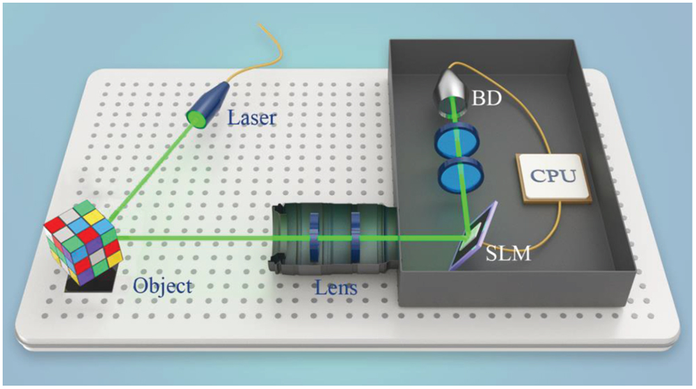
We use a conventional CGI experimental device in our work. The setup is shown in Fig. 1. In the setup, a quasi-monochromatic laser illuminates an object , and the reflected light carrying the object information is modulated by a spatial light modulator. A bucket detector collects the modulated light . Correspondingly, the calculated light can be obtained by diffraction theory. The object image can be reconstructed by correlating the signal output by the bucket detector and calculated signal[
![]()
Figure 1.Setup of the CGI system with CS-CNN. SLM, spatial light modulator; BD, bucket detector.
The flow chart of the CS-CNN is shown in Fig. 2. In the following, we briefly introduce the process of this algorithm. The algorithm mainly consists of three parts: (i) a conventional CS program to compress the data collected by the CGI device; (ii) a conventional CGI process program; and (iii) a 10-layer CNN constructed for the training data.
![]()
Figure 2.Network structure of the proposed CS-CNN.
In the conventional CGI device, a set of data () is measured by a bucket detector. Correspondingly, according to the diffraction theory of light, the distribution of the idle light field in the object plane can be obtained. Thus, we obtain data points. Each data point is divided into blocks without overlapping. According to CS theory[
A new set of data is obtained by processing the above data with a conventional CGI program. Then, a 10-layer CNN is constructed to train the data. Layers 1–4 of the network are stacked autoencoders, and layers 5–10 are convolution layers. The measurement matrix is replaced by a stacked autoencoder, and the input layer is data blocks. All of the rows are arranged into a column vector. If the number of neurons in the first layer is , the measurement rate is . The first layer of the network is connected to the column vector converted from the input image block, and the number of neurons is set according to different measurement rates. The activation function is a rectified linear unit (ReLU) function, which outputs the -dimensional column vector , i.e.,
The second layer of the network is fully connected to the first layer, which has 400 neurons. Take the output of the first layer as the input, output , and the activation function is the ReLU function. In the same way, the third layer is fully connected to the second layer with 100 neurons. The fourth layer is fully connected to the third layer with 400 neurons. The initial reconstructed image block vector is rearranged into image blocks according to the original row and column to obtain the preliminary reconstructed image block.
Finally, the CNN is used to reconstruct the image block accurately. The output data of the fourth layer are taken as the input of the fifth layer. In the fifth layer, sixty-four convolution kernels are used to generate sixty-four feature maps. The sixth layer of the network is connected to the fifth layer (a convolution layer), and thirty-two convolution kernels are used to generate thirty-two characteristic graphs. The seventh layer of the network is connected to the sixth layer (a convolution layer), and a convolution kernel is used to generate a feature map. The eighth layer of the network is connected to the seventh layer (a convolution layer), and sixty-four convolution cores are used to generate sixty-four feature maps. The ninth layer of the network is connected to the eighth layer (a convolution layer), and thirty-two convolution kernels are used to generate thirty-two characteristic graphs. The activation function of the above process is an ReLU function. The tenth layer of the network is connected to the ninth layer (a convolution layer). A convolution kernel is used. The number of zeros in the tenth layer (a convolution layer) is three, and the output of the activation function is not used to generate the reconstructed image block of size .
In the DL framework Caffe, the 10-layer network is trained in an unsupervised way, and the loss function is
The number of input neurons in the first layer is zero, and the number of output neurons in the fourth layer is zero. In the 5th to 10th layers of the network, the initial weight distribution is subject to a Gaussian distribution with a mean of zero and a variance of 0.01. In layers 1–10 of the network, the initial offset values are set to zero. After the deep neural network, the reconstructed image blocks are obtained, then the image blocks are rearranged according to the original row, and the row values are rearranged according to the index.
3. Results
The experimental setup is schematically shown in Fig. 1. A standard monochromatic laser (30 mW, Changchun New Industries Optoelectronics Technology Co., Ltd., MGL-III-532) with wavelength illuminates an object (Rubik’s Cube). The light reflected by the object focuses on a two-dimensional amplitude-only ferroelectric liquid crystal spatial light modulator (Meadowlark Optics A512-450-850) with addressable pixels through the lens. A bucket detector collects the modulated light. Correspondingly, the reference signal is obtained by MATLAB software. The ghost image is reconstructed by the CS-CNN. In this experiment, the sampling rate is , and the number of training sets is 1000.
Figure 3 shows a set of experimental results. Figure 3(a1) is the object. Figures 3(a2)–3(a5) represent reconstructed ghost images with different numbers of frames. The results show that the image quality is significantly improved by increasing the number of frames. High-quality ghost images comparable to classical optical imaging can be produced with little data. To quantitatively analyze the quality of the reconstructed image at different frames, the peak signal to noise ratio (PSNR) and structural similarity index (SSIM) are used as our evaluation indexes. As can be seen from Fig. 3(b), despite the number of samples being very small, the reconstructions are still in reasonable quality.
![]()
Figure 3.Ghost images reconstructed by CGI with CS-CNN. (a1) Classical image. The numbers of frames in the reconstructed ghost images are (a2) 30, (a3) 50, (a4) 70, and (a5) 90. (b) PSNR and SSIM curves of the reconstructed images with different frame numbers.
We compare the conventional CS, DL, and CS-CNN CGI algorithms based on the same experimental data in Fig. 4. CGI can not effectively reconstruct the image when the number of frames is less than 100. Consequently, there is no experimental result of CGI in Fig. 4. The conventional CS algorithm and CS-CNN algorithm have the same sampling rate, i.e., . The DL algorithm and CS-CNN algorithm set the same dataset, i.e., 1000. When the number of samples is very low, Fig. 4 shows that with the same number of frames the image quality obtained by this scheme is the best. The quantitative results (Fig. 5) show that the PSNR of CGI with CS-CNN is on average 28.4% higher than that of CGI with DL under the same reconstructed frame number, and SSIM increases by 93.8% on average[
![]()
Figure 4.Detailed comparison between the ghost images reconstructed using the conventional CS algorithm, DL algorithm, and CS-CNN algorithm. The number of frames is (a) 30, (b) 50, (c) 70, and (d) 90.
![]()
Figure 5.PSNR and SSIM curves of reconstructed images of CS, DL, and CS-CNN with different frame numbers.
4. Summary
In summary, we have proposed a novel method to improve the image quality of CGI. This method combines the advantages of the CS algorithm and CNN algorithm. We analyzed the performance of the conventional CGI, CS, and DL algorithms under the same conditions and observed that our CS-CNN scheme outperforms the other methods, especially when the sampling rate is small. CS based on a CNN is the better CGI method to date. This method provides a promising solution to these challenges that prohibit the use of CGI in practical applications.
References
[1] T. B. Pittman, Y. H. Shih, D. V. Strekalov, A. V. Sergienko. Optical imaging by means of two-photon quantum entanglement. Phys. Rev. A, 52, R3429(1995).
[2] J. Cheng, S.-S. Han. Incoherent coincidence imaging and its applicability in X-ray diffraction. Phys. Rev. Lett., 92, 093903(2004).
[3] X. H. Chen, Q. Liu, K. H. Luo, L. A. Wu. Lensless ghost imaging with true thermal light. Opt. Lett., 34, 695(2009).
[4] B. I. Erkmen. Computational ghost imaging for remote sensing. J. Opt. Soc. A, 29, 782(2012).
[5] D. Y. Duan, Z. X. Man, Y. J. Xia. Nondegenerate wavelength computational ghost imaging with thermal light. Opt. Express, 27, 25187(2019).
[6] J. H. Gu, S. Sun, Y. K. Xu, H. Z. Lin, W. T. Liu. Feedback ghost imaging by gradually distinguishing and concentrating onto the edge area. Chin. Opt. Lett., 19, 041102(2021).
[7] G. Wang, H. B. Zheng, Z. G. Tang, Y. C. He, Y. Zhou, H. Chen, J. B. Liu, Y. Yuan, F. L. Li, Z. Xu. Naked-eye ghost imaging via photoelectric feedback. Chin. Opt. Lett., 18, 091101(2020).
[8] D. Pelliccia, A. Rack, M. Scheel, V. Cantelli, D. M. Paganin. Experimental X-ray ghost imaging. Phys. Rev. Lett., 117, 113902(2016).
[9] H. Yu, R. Lu, S. Han, H. Xie, G. Du, T. Xiao, D. Zhu. Fourier-transform ghost imaging with hard X rays. Phys. Rev. Lett., 117, 113901(2016).
[10] A. Zhang, Y. He, L. Wu, L. Chen, B. Wang. Tabletop X-ray ghost imaging with ultra-low radiation. Optica, 5, 374(2018).
[11] W. Li, Z. Tong, K. Xiao, Z. Liu, Q. Gao, J. Sun, S. Liu, S. Han, Z. Wang. Single-frame wide-field nanoscopy based on ghost imaging via sparsity constraints. Optica, 6, 1515(2019).
[12] W. Gong, S. Han. High-resolution far-field ghost imaging via sparsity constraint. Sci. Rep., 5, 9280(2015).
[13] J. H. Shapiro. Computational ghost imaging. Phys. Rev. A, 78, 061802(R)(2008).
[14] Y. Bromberg, O. Katz, Y. Silberberg. Ghost imaging with a single detector. Phys. Rev. A, 79, 053840(2009).
[15] O. Katza, Y. Bromberg, Y. Silberberg. Compressive ghost imaging. Appl. Phys. Lett., 95, 131110(2009).
[16] V. Katkovnik, J. Astola. Compressive sensing computational ghost imaging. J. Opt. Soc. Am. A, 29, 1556(2012).
[17] P. W. Wang, C. L. Wang, C. P. Yu, S. Yue, W. L. Gong, S. S. Han. Color ghost imaging via sparsity constraint and non-local self-similarity. Chin. Opt. Lett., 19, 021102(2021).
[18] Z. Chen, J. Shi, G. Zeng. Object authentication based on compressive ghost imaging. Appl. Opt., 55, 8644(2016).
[19] M. Lyu, W. Wang, H. Wang, W. Wang, G. Li, N. Chen, G. Situ. Deep-learning-based ghost imaging. Sci. Rep., 7, 17865(2017).
[20] Y. He, G. Wang, G. Dong, S. Zhu, H. Chen, A. Zhang, Z. Xu. Ghost imaging based on deep learning. Sci. Rep., 8, 6469(2018).
[21] T. Shimobaba, Y. Endo, T. Nishitsuji, T. Takahashi, Y. Nagahama, T. Hasegawa, M. Sano, R. Hirayama, T. Kakue, A. Shiraki, T. Ito. Computational ghost imaging using deep learning. Opt. Commun., 413, 147(2018).
[22] G. Barbastathis, A. Ozcan, G. Situ. On the use of deep learning for computational imaging. Optica, 6, 921(2019).
[23] X. L. Yin, Y. J. Xia, D. Y. Duan. Theoretical and experimental study of the color of ghost imaging. Opt. Express, 26, 18944(2018).
[24] W. J. Jiang, X. Y. Li, X. L. Peng, B. Q. Sun. Imaging high-speed moving targets with a single-pixel detector. Opt. Express, 28, 7889(2020).
[25] D. F. Shi, C. Y. Fan, P. F. Zhang, H. Shen, J. H. Zhang, C. H. Qiao, Y. J. Wang. Two-wavelength ghost imaging through atmospheric turbulence. Opt. Express, 21, 2050(2013).
[26] Y. H. Liu, S. Y. Liu, F. X. Fu. Optimization of compressed sensing reconstruction algorithms based on convolutional neural network. Comput. Sci., 47, 143(2020).

Set citation alerts for the article
Please enter your email address
© Copyright 2018-2021 | Chinese Laser Press. All Rights Reserved 沪ICP备15018463号-20