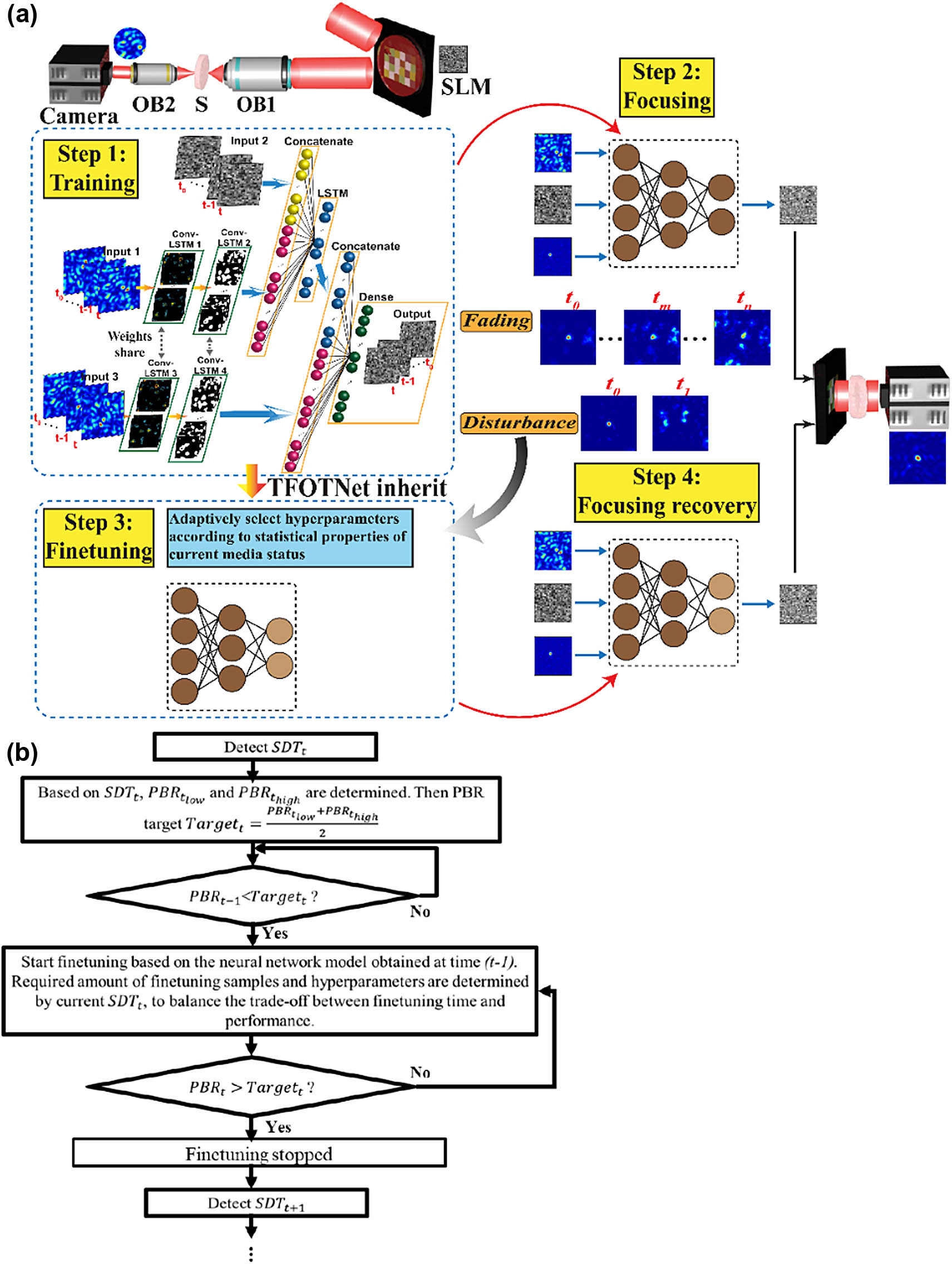
Fig. 1. Illustration of the proposed deep learning-empowered adaptive framework for wavefront shaping in nonstationary media. (a) General working principle of the proposed framework. In Step 1, samples are collected to train the TFOTNet. The structure of the proposed TFOTNet includes three inputs and one output. Input 1 is the speckle pattern, while the corresponding SLM pattern is noted as Input 2. Input 3 is the speckle pattern desired to be seen by the camera after light passes through the scattering medium in the experiment or simulation. TFOTNet output is the SLM pattern needed to get Input 3 through the present scattering medium. In Step 2, the well-trained TFOTNet can be applied to unseen speckles and output an SLM pattern that can obtain the target through the current medium. Inevitable environmental disturbance (disturbance) or nonstationary change in the medium (fading) results in degradation or even loss of the focal point. In Step 3, the pre-trained TFOTNet is fine-tuned with samples from the changing medium. Hyperparameters and fine-tuning sample amount are all adaptively chosen based on the medium status. After tuning, TFOTNet can adapt to the concurrent medium state and recover the optical focusing performance. (b) Flow chart of the proposed adaptive recursive algorithm for light focusing and refocusing in nonstationary media.

Fig. 2. Fine-tuning results with ten random nonstationary processes using three different algorithms. The 10 nonstationary processes can be regarded as consisting of multiple piece-wise stochastically stationary sub-processes, while the SDT and time duration of each sub-process are different. (a)–(j) Fine-tuning results with the adaptive recursive algorithm (gray line), nonadaptive recursive algorithm (red line), and traditional fine-tuning algorithm (blue line) in the 10 nonstationary processes. Each process is characterized by SUMM, which is the sum of the product of SDT of each sub-process and its time duration. Figures (a)–(j) use the same legend. (k) Global focusing performance of three fine-tuning algorithms in the ten random nonstationary processes. (l) Global tracking error of three fine-tuning algorithms in the ten random nonstationary processes. Figures (k) and (l) use the same legend. The inserted table lists the default values of these hyperparameters used in simulation. Specific hyperparameters and fine-tuning sample amounts used in the simulation are available in Ref. [83].

Fig. 3. Schematic of the experimental setup. Light is expanded by two lenses (L1 and L2), and then a half-waveplate (HW) and a polarizer (P) adjust the polarization state of the light incident onto the spatial light modulator (SLM). Light is modulated and reflected by the SLM, then passes through two lenses (L3 and L4), and is focused onto a diffuser (D) surface by an objective lens (OB1). Scattered light is collected by another objective lens (OB2) and recorded by a camera.

Fig. 4. Experimental results. (a) Global focusing performance in the six experiments with the adaptive recursive algorithm and traditional algorithm. (b) Global tracking error in the six experiments with adaptive recursive algorithm and traditional algorithm. Figures (a) and (b) use the same legend. (c) The enhancement percentage in global focusing performance achieved by the adaptive recursive algorithm over the traditional algorithm. (d) The reduction percentage in global tracking error achieved by the adaptive recursive algorithm over the traditional algorithm.

Fig. 5. (a)–(c) Experimental results of the three trials without environmental disturbance. The SDT of each stationary sub-process is shown in the figure, and the PBR target (ideal case) is indicated by yellow dashed lines. (d)–(f) Results of the three experiments with environmental disturbance. Figures (a)–(f) use the same legend. (g) Speckle images recorded during a nonstationary process with environmental perturbation using adaptive recursive and traditional algorithms. In (g), all speckle images use the same colormap and scale and are interpolated to 253×253 for a better view. The color bars indicate the detected light intensity in arbitrary units. The middle image in the bottom row (traditional fine-tuning) is an interpolated result using recorded speckles. Specific hyperparameters and fine-tuning sample amount used in experiments are available in Ref. [83].

Fig. 6. Comparisons about fine-tuning ability in a nonstationary process using three different networks (see Visualization 1). (a) Simulation results. Light focusing and refocusing performance recorded at different times through a nonstationary process using the adaptive recursive algorithm with TFOTNet (the first row), ConvLSTM (the second row), and CNN (the third row) is shown. All images use the same colormap and scale, and the color bars indicate the light intensity in arbitrary units. (b) Experimental results. Light focusing and refocusing results using three networks with the adaptive recursive algorithm in the same nonstationary process are shown. All speckle images use the same colormap and scale and are interpolated to 253×253. The color bars indicate the detected light intensity in arbitrary units. (c) Experimental results in the situation of low SNR. All speckle images use the same colormap and scale and are interpolated to 253×253. The color bars indicate the detected light intensity in arbitrary units. (d) Structure of a conventional single-input-single-output ConvLSTM. (e) Structure of a conventional single-input-single-output CNN. (f) Details of the nonstationary process and PBR with the three networks in simulation (a). (g) Details of the nonstationary process and PBR with the three networks in experiment (b). (h) Details of the nonstationary process and PBR with the three networks in experiment (c). (f)–(h) use the same legend.

Fig. 7. Influence of hyperparameters on fine-tuning time cost and performance when the scattering medium changes at various speeds. (a)–(d) The effect of sample amount, timestep, batch size, and initial learning rate on fine-tuning time cost under five circumstances where the scattering medium is changing at different speeds (indicated by lines of different colors and quantified by speckle decorrelation time). (e) The required amount of fine-tuning samples with and without adaptive adjustments of hyperparameters as the medium changes at different speeds. (f), (g) The relationship between the PBR after fine-tuning and the fine-tuning sample amount using the adaptive algorithm as the medium changes at different speeds. The default values of these hyperparameters used in the simulation are listed in Fig. 2.

Table 1. SDT-Dependent PBR Target